Quickly Create Summary Worksheet with Hyperlinks in Excel

A lot of my colleagues spend a lot of their time in creating a Summary Worksheet in Excel.

A typical summary worksheet has the names of all the worksheets in different cells and all the names also hyperlinked to these worksheets.

So you can click on a cell with a sheet name (say Jan, Feb, Mar…) and it will take you to that worksheet. Additionally, there is also a hyperlink on each worksheet that links back to the summary worksheet.

While my colleagues have become super efficient in doing this, it’s still a waste of time when you can do the same thing in less than a second (yes you read it right).

The trick is to create a short macro that will do it for you.

No matter how many worksheets you have, it will instantly create a summary worksheet with working hyperlinks.

Something as shown below:

As you can see in the image above, it instantly creates the summary when you run the macro (by clicking on the button). The sheet names are hyperlinked which takes you to the worksheet when you click on it.

Create Summary Worksheet with Hyperlinks

All the heavy lifting in creating the summary worksheet is done by a short VBA code. You just need to run the code and take a break as you would have some free time now 🙂

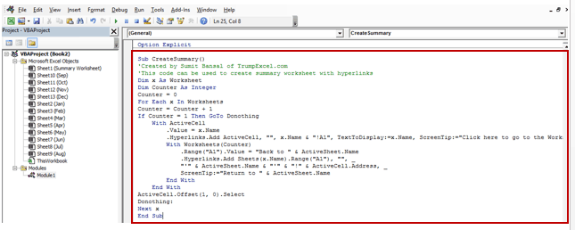
Here is the code:

Sub CreateSummary()
'Created by Sumit Bansal of trumpexcel.com
'This code can be used to create summary worksheet with hyperlinks
Dim x As Worksheet
Dim Counter As Integer
Counter = 0
For Each x In Worksheets
Counter = Counter + 1
If Counter = 1 Then GoTo Donothing
    With ActiveCell
        .Value = x.Name
        .Hyperlinks.Add ActiveCell, "", x.Name & "!A1", TextToDisplay:=x.Name, ScreenTip:="Click here to go to the Worksheet"
        With Worksheets(Counter)
            .Range("A1").Value = "Back to " & ActiveSheet.Name
            .Hyperlinks.Add Sheets(x.Name).Range("A1"), "", _
            "'" & ActiveSheet.Name & "'" & "!" & ActiveCell.Address, _
            ScreenTip:="Return to " & ActiveSheet.Name
        End With
    End With
ActiveCell.Offset(1, 0).Select
Donothing:
Next x
End Sub

Where to Put this Code?

Follow the steps below to place this code in the workbook:

1. Go to Developer Tab and Click on Visual Basic. You can also use the keyboard shortcut – ALT F11.
   • If you can find the developer tab in the ribbon in Excel, click here to know how to get it.
2. There should be a Project Explorer pane at the left (if it is not there, use Control + R to make it visible).
3. Go to Insert and Click in Module. This adds a module to the workbook. Also, in the right, you would see the code window appears (with a blinking cursor). 
4. In the module code window, copy and paste the above code.

Running the Code

To run this code:

• Go to Developer Tab –> Code –> Macros. This will open the Macro Dialogue box.
• Select the Macro CreateSummary and click on Run.
• This will run the macro and create the hyperlinks in the active sheet.

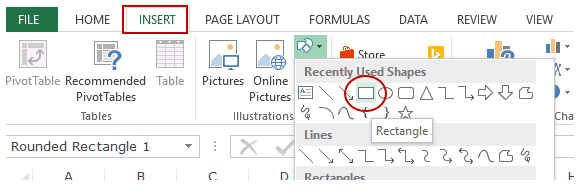
Another way to run the macro is to insert a button/shape and assign the macro to it. To do this:

• Insert a shape in the worksheet. Format the shape the way you want.
• Right-click on it and select Assign Macro.
• In the Assign Macro box, select the macro you want to assign to the shape and Click OK.

Now, you can simply click on the shape to run the macro.

Download the File from here

Note:

1. I have hard-coded the cell A1 in each sheet, which is hyperlinked to get you back to the summary sheet. Ensure that you change it accordingly if you have something already in A1 cell in each sheet.
2. The summary does not create a hyperlink for itself (which makes sense as you are already on that sheet).
3. Run this code when the Summary Worksheet is the active worksheet.
4. You may want to add some formatting or rearrangement. But I hope this code takes care of the hard part.
5. Save this workbook as .xls or .xlsm extension, as it contains a macro.

Other Excel VBA tutorials:

• Get Multiple Lookup Values Without Repetition in a Single Cell.
• Task Prioritization Matrix – VBA Application.
• How to Combine Multiple Workbooks into One Excel Workbook.
• Excel VBA Loops – For Next, Do While, Do Until, For Each (with Examples).
• How to Record a Macro in – A Step by Step Guide.
• How to Quickly Remove Hyperlinks from a Worksheet in Excel.
• Online Excel VBA Course.
• How to Switch Between Sheets in Excel?