How to Print Excel Sheet on One Page (Fit to One Page)

If you often print your data/work in Excel, I am sure you have faced the issue where it prints multiple pages instead of one single page.

Sometimes, it’s so frustrating that a new page is printed just to accommodate a few extra lines of data (which also leads to wastage of paper).

There are some simple techniques you can use to make sure you Excel data in printed on one page (or in less number of pages in case you’re printing a big report).

In this Excel tutorial, I will share some methods you can use to print the Excel sheet on one page. You can use a combination of these methods to get the best result.

So let’s get started!

Check How Many Pages Would be Printed (Preview)

Before you set out to optimize the settings to print the Excel work in one sheet, it’s best to check the current state using the Print Preview.

Don’t worry! You don’t have to print anything for this. You can simply check how the printed work would look and how many sheets will be printed.

This allows you to understand the things you can change to make sure you’re using the minimal number of paper while still keeping your printed report beautiful and legible.

Below are the steps to use Print Preview to see how the final print job would look like:

1. Click the File tab
2. Click the Print Option

Or you can use the keyboard shortcut Control + P (Command + P if using a Mac)

This would open the Print preview page where you would be able to see how many pages would be printed and what would be printed on each page.

You can use the arrow keys to go to the next/previous page when in the Print preview mode.

Ways to Fit and Print Excel Sheet in One Page

Now, let’s see some methods you can use to fit all the data in a sheet on one page and then print your report on one page (or fewer number of pages)

Adjust the Column Width (or Row height)

In many cases, you don’t need your columns to be too wide.

And since this is a direct determinant of how much data is printed on one page, you can save a lot of paper by simply reducing the column width.

But then, how do you know whether you have done enough or not? How do you know how much column width you should reduce to make everything fit on one page?

To make this easy, you can use the Page Layout View in Excel – which shows you in real-time how much data would be printed on each page of your report.

Below are the steps to get into the Page Layout mode and then reduce the column width:

1. Click the View tab in the ribbon
2. In the Workbook Views group, click on the ‘Page Layout’ option. This will change the way data is displayed (and you will see scales at the top and on the left of the worksheet)
3. Reduce the column width to fit the data on one page. To do this, place the cursor at the edge of the cursor on the column header that you want to reduce in size. Then click and drag.

Once you have all the data on one page, you can go ahead and print it.

In some cases, you may find that the data in a cell is being cut off and is not being displayed completely. This often happens when you change the column width. You can correct this by enabling the Wrap text option in Excel.

To return to the normal view (and get out of the Page Layout view), click on the View tab and then click on ‘Normal’.

Change the Scaling (Fit All Rows/Columns in One Page)

Excel has an in-built option that allows you to rescale the worksheet in a way that fits more rows/columns on one page.

When you do this, it simply scales down everything to fit all the columns or rows in one page.

Suppose you have a sheet where the columns are spilling over to the next sheet when printed.

Below are the steps to scale down the sheet while printing:

1. Click the File tab
2. Click on Print (or use the keyboard shortcut – Control + P)
3. In the Print window, click on the Scaling option (it’s the last option on the left)
4. Click on any one of the options:
   • Fit Sheet on One Page
   • Fir All Columns on One Page
   • Fit All Rows on One Page

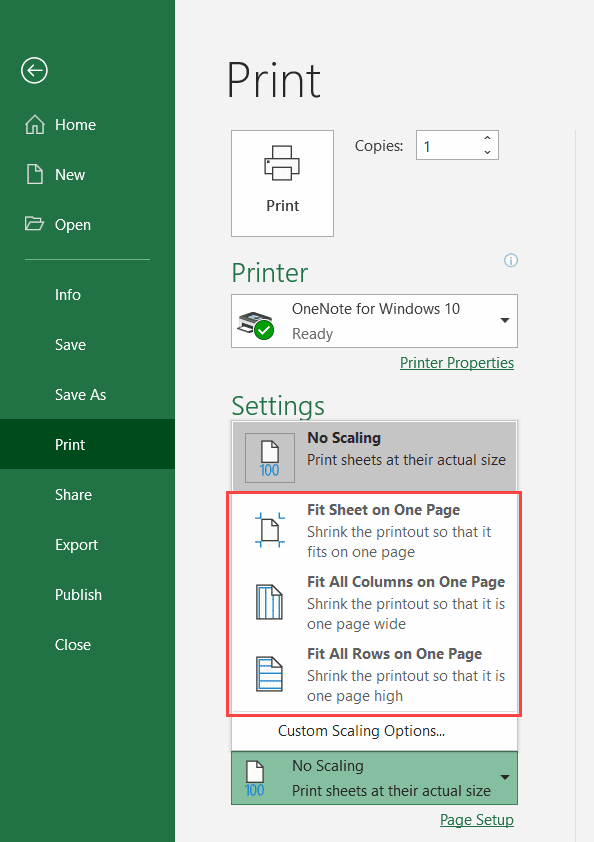
The above steps would scale the sheet to fit the page (based on what options you have selected). You will also be able to see how the data would look in the sheet preview which is on the right.

This doesn’t impact the worksheet data. It only scales the data for print purposes.

Hide or Delete Rows/Columns

Another smart way to get everything on one page when printing is to hide any columns or rows that you don’t need.

You always have the option to make these visible again in case you need it later, but hiding these while printing will make sure you’re optimizing the space and using fewer pages to print.

To hide a row/column, simply select them, right-click and then select Hide.

Again, it’s best to first get into the Page Layout mode and then do this. This makes sure you can see how many rows/columns you need to hide to fit all the data on one page in Excel.

And here are steps to unhide the rows/columns in Excel.

Change the Page Orientation

If you have more columns and rows, it makes sense to change the orientation of the page while printing.

There are two Orientations in Excel;

• Portrait (default in Excel) – More rows are printed than columns
• Landscape – More columns are printed than rows

In case you have more columns than rows (as shown below), you can change the page orientation to Landscape to ensure your data fit and is printed on one page.

Below are the steps to change the page orientation in Excel:

1. Click the Page Layout tab
2. In the Page Setup group, click on the dialog box launcher. This will open the ‘Page Setup’ dialog box.
3. Click on the Page tab in the dialog box (if not selected already)
4. In the Orientation option, select Landscape
5. Click OK

Now you can go to Print Preview and see how your printed report would look like.

The keyboard shortcut to open the Page Setup dialog box ALT + P + S + P (press these keys in succession)

Alternatively, you can also change the orientation in the Print Preview window, by selecting Landscape Orientation from the drop-down in the settings.

Change the Page Margins

Sometimes you just have one or two extra columns that are getting printed on a new page (or a few extra rows that are spilling to the next page).

A little adjustment in the Page margins may help you fit everything on a single page.

If you’re wondering what page margins are – when you print an Excel worksheet, every printed page would have some whitespace at the edges. This is by design to make sure the data looks good when printed.

You have the option to reduce this white space (the page margin) and fit more data on a single page.

Below are the steps to reduce the page margin in Excel:

1. Click the Page Layout tab
2. In the Page Setup group, click on ‘Margins’
3. Click on Narrow

The above steps would reduce the page margin and you may see some extra rows/columns being squeezed on the same page.

In case you want to further reduce the page margin, click on the ‘Margins’ option in the ribbon, and then click on ‘Custom Margins’. This will open the Page Setup Dialog box where you can further adjust the margins.

Reduce the Font Size

Another simple way to quickly make some extra rows/columns (that are spilling to additional sheets when printed as of now) fit the same page can be by reducing the font size.

This can allow you to resize a few columns so that it fits one page when printed.

This can be useful when you have printed data that usually goes in the appendix – something you need to have but nobody reads or cares about it.

Print Selected Data only (or Set the Print Area)

Sometimes, you may have a large dataset, but you may not want to print all of it. Maybe you only want to print selected data.

If this is a one-off thing where you want to quickly print the selected data in the worksheet, you can do that using the below step:

1. Select the data that you want to print
2. Click the File tab
3. Click on Print (or use the keyboard shortcut – Control + P)
4. In the Print screen that shows up, click on the first option in Settings
5. Click on the Print Selection option. You would notice that the preview also changes to show you only the part that would be printed.
6. Click on Print.

The above steps would only print the selected dataset.

Note that in case you selected a dataset that can’t be fit into a single plage when printed, it will be printed on multiple sheets. You can, however, change the scaling to ‘Fit Sheet on One Page’ to print selection on a single page.

The above method is good when you have to print the selected data once in a while.

But you need to print the same selection from multiple worksheets, it’s a better idea to set the print area. Once set, Excel would consider this Print Area as the part that is meant to print and would ignore the other data on the sheet.

Below are the steps to set the print area in Excel:

1. Select the data that you want to set as the print area
2. Click the Page Layout tab
3. In the Page Setup group, click on the Print Area option
4. Click on Set Print Area

That’s it!

Now when you try and print a worksheet, only the print area would be printed (and only this will be shown in the Print Preview).

[Bonus] Add Page Breaks

In case you have a large dataset. it’s obvious that it can not be fit into one page and printing this entire data would take up multiple pages.

You can add page breaks in Excel to let Excel know where to stop printing on the current page and spill the rest to the next page.

Below are the steps to add page breaks in Excel:

1. Select the cell where you want to insert the page break. From this cell onwards, everything would be printed on the next page
2. Click the Page Layout tab
3. In the Page Setup group, click on Breaks option
4. Click on Insert Page Breaks

The above steps would add a page break and everything before the page break would be printed in one sheet and the remaining data in other sheets.

Note that in case you have set the print area, it will take precedence over page breaks.

So these are various methods you can use to fit data into one page and print an Excel spreadsheet on one page. In cases where you have a lot of data, it may not make sense to print it on one page, but you can still use the above methods to minimize paper usage and fit the same data into fewer pages.

I hope you found this tutorial useful.

You may also like the following Excel tutorials:

• How to Print Comments in Excel
• How to Print the Top Row on Every Page in Excel
• How to Print Multiple Sheets (or All Sheets) in Excel in One Go
• How to Unhide COLUMNS in Excel
• How to Group Worksheets in Excel
• How to Compare Two Excel Sheets (for differences)