
When you enter a text string in Excel which exceeds the width of the cell, you can see the text overflowing to the adjacent cell(s).
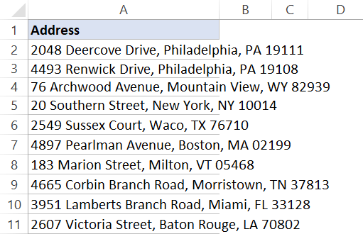
Below is an example where I have some address in column A and these address overflow to the adjacent cells as well.
And in case you have some text in the adjacent cell, the otherwise overflowing text would disappear and you will only see the text that can fit the cell column width.
In both cases, it doesn’t look good and you may want to wrap the text so that the text remains within a cell and not spill over to others.
This can be done using the wrap text feature in Excel.
In this tutorial, I will show you various ways of wrapping text in Excel (including doing it automatically with a single click, using a formula and doing it manually)
So let’s get started!
Wrap text with a Click
Since this is something you may need to do quite often, there is easy access to quickly wrap the text with a click on a button.
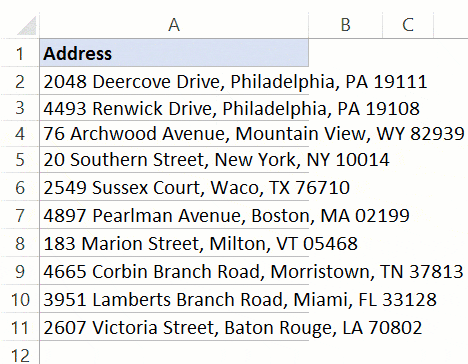
Suppose you have the dataset as shown below where you want to wrap text in column A.
Below are the steps to do this:
- Select the entire dataset (column A in this example)
- Click the Home Tab

- In the Alignment group, click on the ‘Wrap text’ button.

That’s It!
All it takes it two-click to quickly wrap the text.
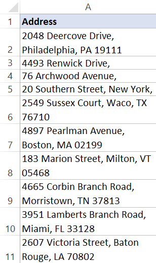
You will get the final result as shown below.
You can further bring down the effort from two to one-click by adding the Wrap text option to the Quick Access Toolbar. To do this. right-click on the Wrap text option and click on ‘Add to Quick Access Toolbar’
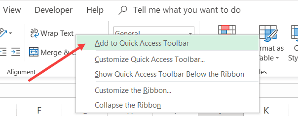
This adds an icon to the QAT and when you want to wrap text in any cell, just select it and click this icon in the QAT.
Also read: How to Make Cells Bigger in Excel?
Wrap text with a Keyboard Shortcut
If you’re like me, leaving the keyboard and using a mouse to click even a single button could feel like a waste of time.
The good news is that you can use the keyboard shortcut below to quickly wrap text in all the selected cells.
ALT + H + W (ALT key followed by the H and W keys)
Wrap text with the Format Dialog box
This is my least preferred method, but there is a reason I am including this one in this tutorial (as it can be useful in one specific scenario).
Below are the steps to wrap the text using the Format dialog box:
- Select the cells for which you want to apply the wrap text formatting
- Click the Home tab
- In the Alignment group, click on the Alignment Setting dialog box launcher (it’s a small ’tilted arrow in a box’ icon at the bottom right of the group).

- In the ‘Format Cells’ dialog box that opens, select the Alignment tab (if not selected already)
- Select the Wrap text option

- Click OK.
The above steps would wrap the text in the selected cells.
Now, if you’re thinking why to use this twisted long method when you can use a keyboard shortcut or a single click on the ‘Wrap Text’ button in the ribbon.
In most cases, you should not be using this method, but it can be useful when you want to change a couple of formatting settings. Since the Format Dialog box gives you access to all the formatting options, this may end up saving you some time.
NOTE: You can also use the keyboard shortcut Control + 1 to open the ‘Format Cells’ dialog box.
How Does Excel Decide How Much text to Wrap
When you use the above method, Excel uses the column width to decide how many lines you get after wrapping.
Doing this makes sure that anything that you have in the cell is confined within the cell itself and doesn’t overflow.
In case you change the column width, the text will also adjust to ensure it fits the column width automatically.
Inserting Line Break (Manually, Using Formula, or Find and Replace)
When you apply ‘Wrap Text’ to any cell, Excel determines the line breaks based on the width of the column.
So if there is text that can fit in the existing column width, it will not be wrapped, but in case it can not, Excel will insert the line breaks by first fitting the content in the first line and then moving the rest to the second line (and so on).
By entering a line break manually, you force Excel to move the text to the next line (in the same cell) right after the line break is inserted.
To enter the line break manually, follow the steps below:
- Double-click on the cell in which you want to insert the line break (or press F2). This will get you into edit mode in the cell
- Place the cursor where you want the line break.
- Use the keyboard shortcut – ALT + ENTER (hold the ALT key and then press Enter).
Note: For this to work, you need to have Wrap Text enabled on the cell. If Wrap Text is not enabled, you will see all the text in one single line, even if you have inserted the line break.
You can also use a CHAR formula to insert a line break (as well as a cool Find and Replace trick to replace any character with a line break).
Both of these methods are covered in this short tutorial on inserting line breaks in Excel.
And in case you want to remove line breaks from cells in Excel, here is a detailed tutorial about it.
Handling Wrapping Too Much Text
Sometimes you may have a lot of text in a cell and when you wrap the text, it may end up making your row height large.
Something as shown below (the text is taken for bookbrowse.com):
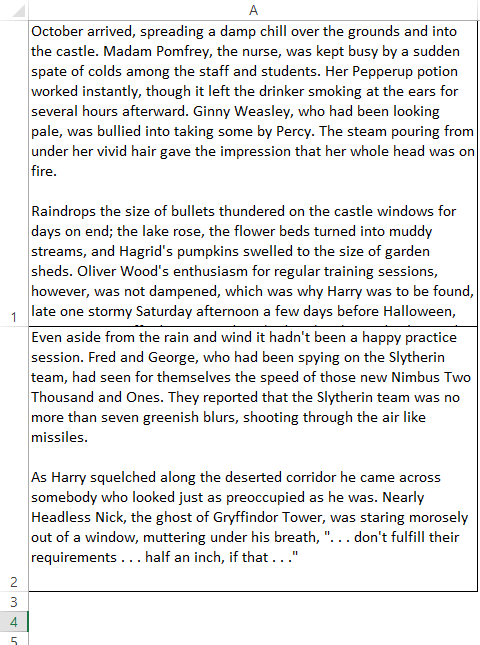
In such a case, you may want to adjust the row height and make it consistent. The downside of this is that not all the text in the cell will be visible, but it makes your worksheet a lot more usable.
Below are the steps to set the row height of the cells:
- Select the cells for which you want to change the row height
- Click the ‘Home’ tab
- In the Cells group, click on the ‘Format’ option

- Click on Row Height

- In the ‘Row Height’ dialog box, enter the value. I am using the value 40 in this example.

- Click OK
The above steps would change the row height and make it all consistent. In case any of the selected cells have text that can not be fit in a cell with the specified height, it will be cut from the bottom.
Don’t worry, the text would still be in the cell. It just won’t be visible.
Also read: Clip Text in Excel
Excel Text Wrap Not Working – Possible Solutions
In case you find that the Wrap text option is not working as expected and you still see the text as a single line in the cell (or with some missing text), there could be a few possible reasons:
Wrap Text is not enabled
Since it works as a toggle, quickly check whether it’s enabled or not.
If it’s enabled, you will see that this option is highlighted in the Home tab
Cell height needs to be adjusted
When Wrap Text is applied, it moves the extra lines below the first line in the cell. In case your cell row height is less, you may not see the entire wrapped text.
In that case, you need to adjust the cell height.
You change the row height manually by dragging the bottom edge of the row.
Alternatively, you can use the ‘AutoFit Row Height’. This option is available in the ‘Home’ tab in ‘Format’ options.
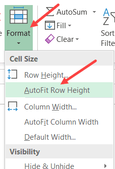
To use the AutoFit option, select all the cells that you want to auto-fit and click on the AutoFit Row Height option.
The Column Width is Already Wide enough
And sometimes there is nothing wrong.
When your column width is wide enough, there is no reason for Excel to wrap the text as it already fits the cell in a single line.
In case you still want the text to split into multiple lines (despite having enough column width), you need to insert the line break manually.
Hope you found this tutorial useful.
You may also like the following Excel tutorials:


Wrap Text is not enabled
Since it works as a toggle, quickly check whether it’s enabled or not.
If it’s enabled, you will see that this option is highlighted in the Home tab
Above is not clear as to how we can ensure edit mode and wrap text are enabled at the same time. Please if you explain with example.
thanks and regards