How to Add Bullet Points in Excel (Shortcut + 7 More Ways)

You can easily add bullet points in a cell in Excel (Yes.. easily).

Until I knew this trick, I used to put a dash (-) or arrow greater than (>>) at the beginning of the text, and that could sometimes be a pain.

I always wondered why was Excel devoid of such basic functionality.

But that was just my ignorance. There is not one, but many ways to add bullet points in a cell in Excel.

In this tutorial, you’ll learn the Windows and Mac shortcuts, formulas for adding bullets to a whole list, and ways to make bullets appear automatically.

While all these methods are quite simple, you only need to know a couple to get your work done.

Bullet Point Shortcut in Excel (Windows and Mac)

You can quickly insert bullet points in Excel using the following keyboard shortcuts.

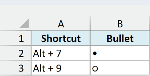
Shortcut on Windows: Alt + 7 or Alt + 9 (using the numeric keypad).

If you have a numeric keypad on your keyboard:

1. Select the cell in which you want to insert the bullet.
2. Double-click on the cell or press F2 to get into edit mode.
3. Hold the Alt key, press 7 or 9 on the numeric keypad, and then leave the Alt key.

As soon as you leave the Alt key, a bullet appears.

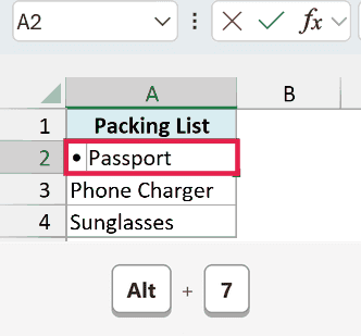
Alt + 7 and Alt + 9 both insert a different kind of bullet.

Without a numeric keypad

If you do not have a numeric keyboard (like my laptop), activate the NumLock first and then repeat the above steps (or try with ALT + FUNCTION + 7)

This works only on laptops with number keys built into the letter keys. Look for small numbers printed on keys like J, K, L, U, I, and O.

If yours has none, copy a bullet from this article, use the Symbol dialog box, or use the formula method below.

Multiple bullet points in one cell

If you want to insert more bullet points in the same cell, repeat the same steps while editing that cell:

1. Enter the bullet followed by the item name.
2. Press Alt + Enter to insert a line break.
3. Insert the bullet again and type the next item.

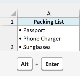
Once you have the bullet in a cell, you can copy it like any other character.

On Mac

In Excel on a Mac, press Option + 8 while editing the cell to insert a bullet.

This works with the U.S. or ABC keyboard layout. On other layouts, Option + 8 can give you a different character.

For more than one bullet in a cell on a Mac, insert a new line between items using the instructions in the article below.

Also read: Start New Line in Excel Cell

See Also: 200+ Excel Keyboard Shortcuts

Pro Tip: Add an AutoCorrect entry that replaces BULSYM with •. Then typing BULSYM gives you a bullet.

Copy and Paste a Bullet Point

If you don’t want to remember a shortcut, you can copy a bullet point from the row below and paste it into Excel.

• ◦ ▪ ■ ○ ● ‣ ➤ ✓

Select the character you want and press Control + C.

Then double-click on the cell in Excel (or press F2) and press Control + V.

A pasted bullet is plain text, so you can change its size and color like any other text.

If you need a tick mark instead, see how to insert a check mark in Excel.

Insert Bullet Points Using the Symbol Dialog Box

You can also use the Insert Symbol option to choose a bullet without a numeric keypad.

Here are the steps:

1. With the cell where you want the bullet selected, go to Insert > Symbols > Symbol.

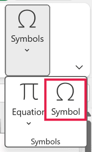
2. In the Symbol dialog box, within the Symbols tab, select the Font.

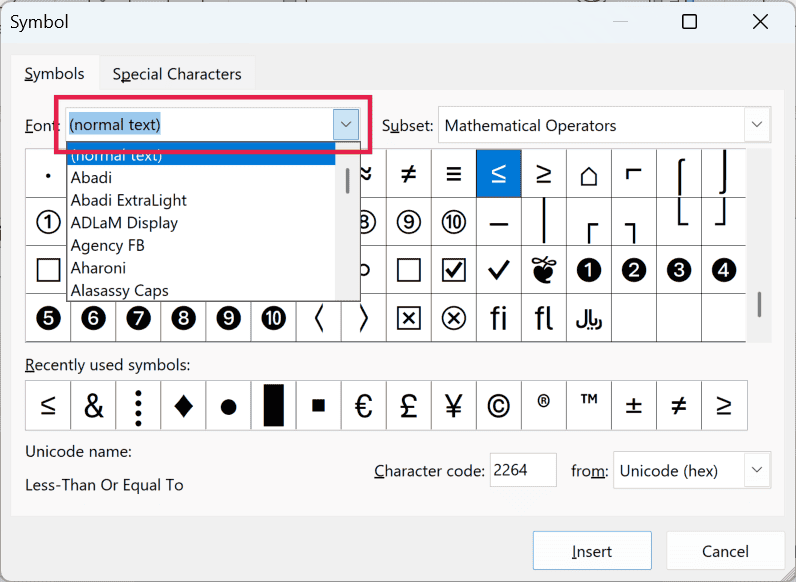
3. Scroll down the symbols list and select the bullet you want to insert.

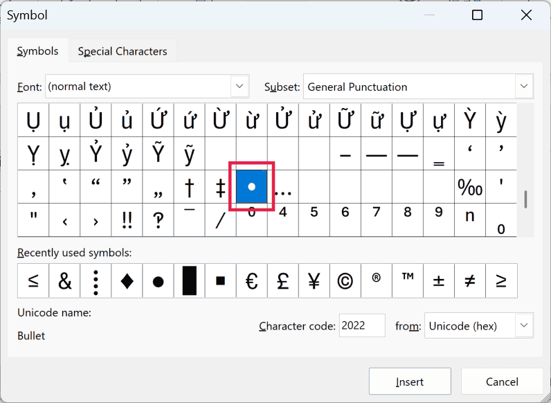
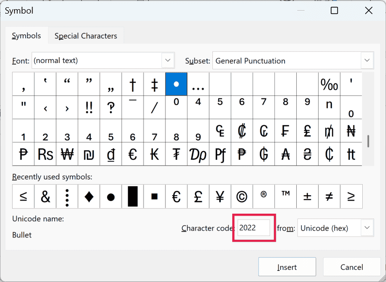
For a faster way to select •, set the “from” drop-down to Unicode (hex) and type 2022 in the Character code box.

If the bullet doesn’t show in your font, choose Wingdings and enter character code 159 instead.

4. Click Insert, then Close.

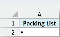
This will insert the bullet in the selected cell. Once you have the bullet in a cell, you can copy-paste it wherever you need it.

Add Bullets to a List Using UNICHAR

A formula is useful when you have a list of items and want to add a bullet to all of them in one go.

Below I have a packing list, and I want to add a bullet before each item in column B.

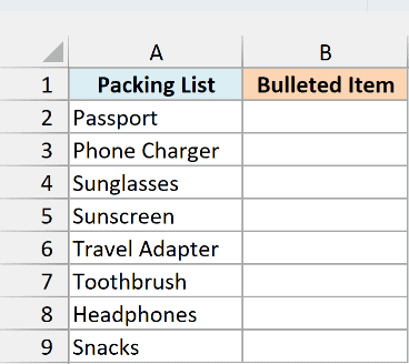
The packing list contains Passport, Phone Charger, Sunglasses, Sunscreen, Travel Adapter, Toothbrush, Headphones, and Snacks.

Enter this formula in B2:

=UNICHAR(8226)&" "&A2:A9

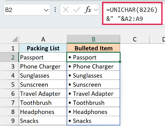
The formula spills down to B9 automatically, giving you “• Passport” through “• Snacks”. You don’t need to copy it down or press Control + Shift + Enter.

UNICHAR(8226) returns the bullet. The number 8226 is the bullet’s Unicode code.

The space character ensures there is space after the bullet and before the item name. The & symbols join the bullet, space, and item together.

The spilling version needs Excel for Microsoft 365 or Excel 2021 and later.

For older versions of Excel

In Excel 2013 through Excel 2019, put this formula in B2 and copy it down to B9:

=UNICHAR(8226)&" "&A2

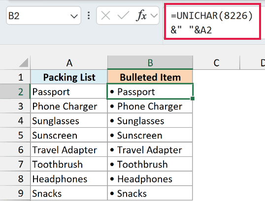
The UNICHAR function needs Excel 2013 or later, so this formula won’t work in earlier versions.

A note about CHAR on Windows

The following formula also returns a bullet on Windows:

=CHAR(149)

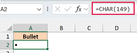
The CHAR function uses your system’s character set, so CHAR(149) doesn’t give you a bullet on a Mac.

The UNICHAR(8226) formula works in Excel 2013 and later on Windows, and in Excel 2021 and later or Microsoft 365 on Mac.

That’s why the list formula above uses UNICHAR(8226).

Also read: Insert Arrows in Excel

Create a Bulleted List in One Cell with TEXTJOIN

If your items are already in separate cells, you can use a formula to put the whole bulleted list in one cell.

Below I have six agenda items, and I want to combine them into a bulleted list in A10.

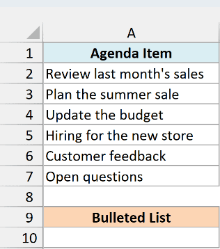
The agenda items are Review last month’s sales, Plan the summer sale, Update the budget, Hiring for the new store, Customer feedback, and Open questions.

Enter this formula in A10:

=UNICHAR(8226)&" "&TEXTJOIN(CHAR(10)&UNICHAR(8226)&" ",TRUE,A2:A7)

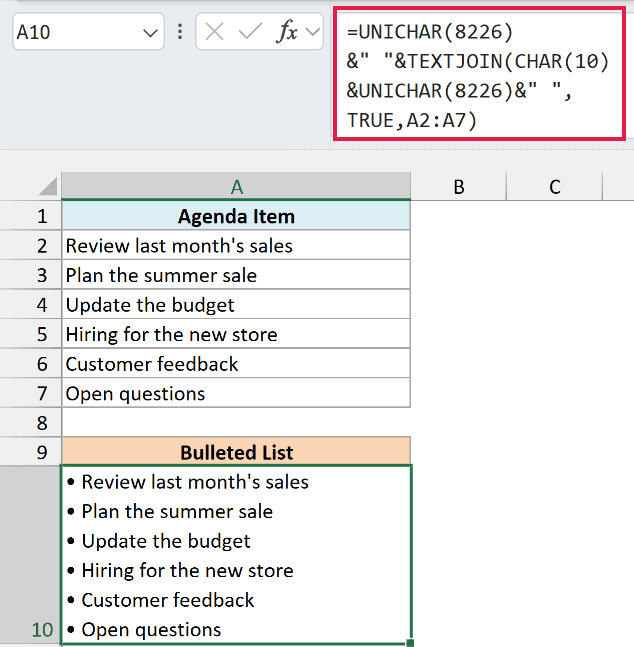
All six items appear inside A10, each on its own line starting with a bullet and a space.

1. Select A10 and turn on Wrap Text from the Home tab > Alignment group > Wrap Text.

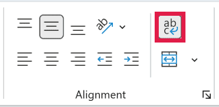
The cell needs Wrap Text turned on. Otherwise, everything shows on one line.

How this formula works:

• TEXTJOIN joins the items in A2:A7.
• Its delimiter is CHAR(10), a line break, followed by a bullet and a space. So every item after the first starts on a new line with its own bullet.
• The UNICHAR(8226)&” ” at the start adds the bullet and space for the first item.
• TRUE tells TEXTJOIN to skip blank cells, so an empty row in the list doesn’t leave a stray bullet.

You need Excel 2019 or later, or Microsoft 365, to use the TEXTJOIN function.

For other ways to join cells, see how to combine cells in Excel.

Make Bullets Appear Automatically with Custom Number Formatting

This one is awesome. You can use custom number formatting to automatically insert bullets in Excel as soon as you enter anything in a cell.

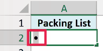
Something as shown below:

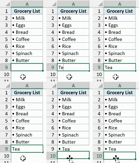
Magic. Isn’t it?

Well… Sort of 🙂

What’s working here in the back end is a nifty custom number formatting trick.

Before I get to the trick, here is what you need to know about custom number formatting in Excel.

It allows you to specify the format for four kinds of data:

<Positive numbers>;<Negative numbers>;<Zeroes>;<Text>

Using custom number formatting, you can specify how each of these data types would be displayed in the cell.

Using this, I can customize cells so that a bullet is automatically displayed as soon as you enter anything in it.

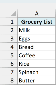
Below I have a grocery list of Milk, Eggs, Bread, Coffee, Rice, Spinach, and Butter, and I want each item in column A to show a bullet.

Here are the steps to apply the format:

1. Get a bullet using the shortcut or Symbol dialog above, or copy • from this article with Control + C. If it’s in a cell, double-click on the cell or press F2, select the bullet, and copy it.

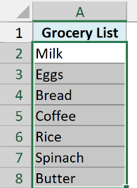
2. Select the cells where you want bullets to appear automatically. For this grocery list, select A2:A8.

3. Press Control + 1 to open the Format Cells dialog box.

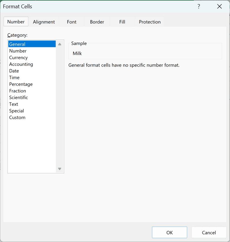
4. In the Number tab, select Custom.

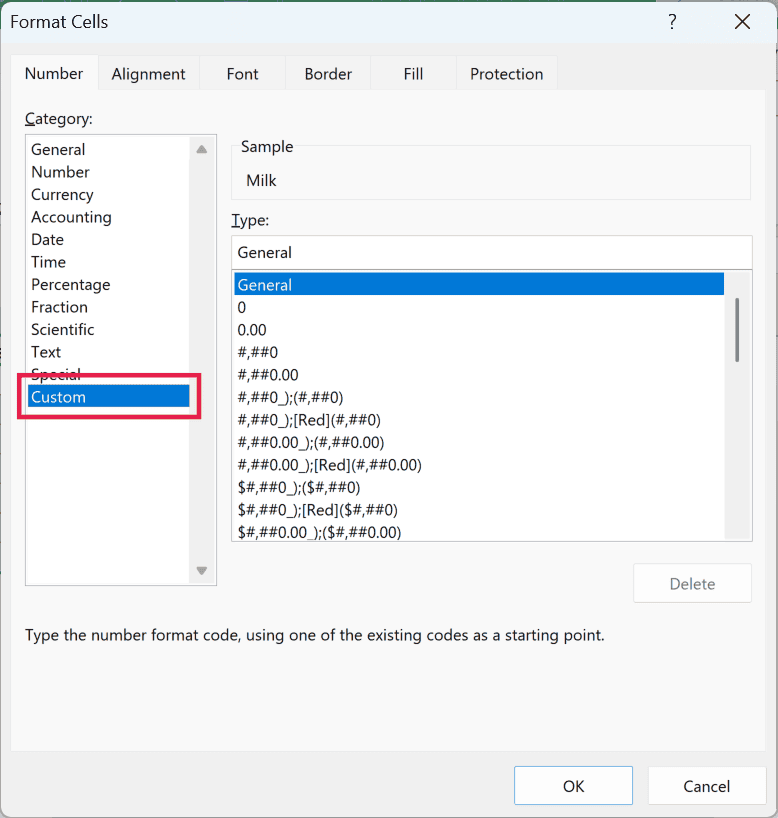
5. In the Type field, enter the following custom number format.

• General;• -General;• General;• @

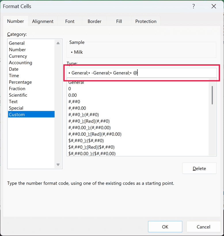
6. Click OK.

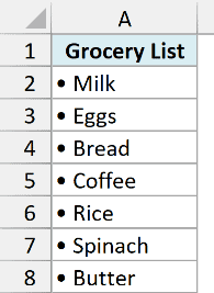
That’s it. Go to the cells and try entering anything. It will automatically show the bullet at the beginning.

The four sections in this custom number format handle positive numbers, negative numbers, zeroes, and text.

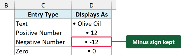
The negative section includes a minus sign so negative numbers keep their sign when the bullet appears.

The @ symbol is the standard placeholder for text, so the last section adds a bullet before text entries.

The old format, • General;• General;• General;• General, had no minus sign in its negative section.

Important: The old format showed -12 as “• 12”. Keep -General in the second section so it shows “• -12”.

Below you can see how all four entry types (a positive number, a negative number, zero, and text) display with this format:

• Text: Olive Oil shows as “• Olive Oil”.
• Positive Number: 12 shows as “• 12”.
• Negative Number: -12 shows as “• -12”.
• Zero: 0 shows as “• 0”.

The bullet is only how the cell looks. A2 still holds just “Milk”, which you can check in the formula bar.

Sorting, filtering, lookups, and formulas work on the real text. With the formula method, the bullet becomes part of the text.

Also read: Insert Symbols in Excel

Copy a Bulleted List from MS Word or PowerPoint

You can easily copy and paste a list with bullet points from MS Word into Excel.

You can paste it in a single cell or get each bullet point in a different cell. Word and PowerPoint lists behave a bit differently when pasted into Excel.

Copy bullet points into a single cell

1. Copy the bullet points from Word.

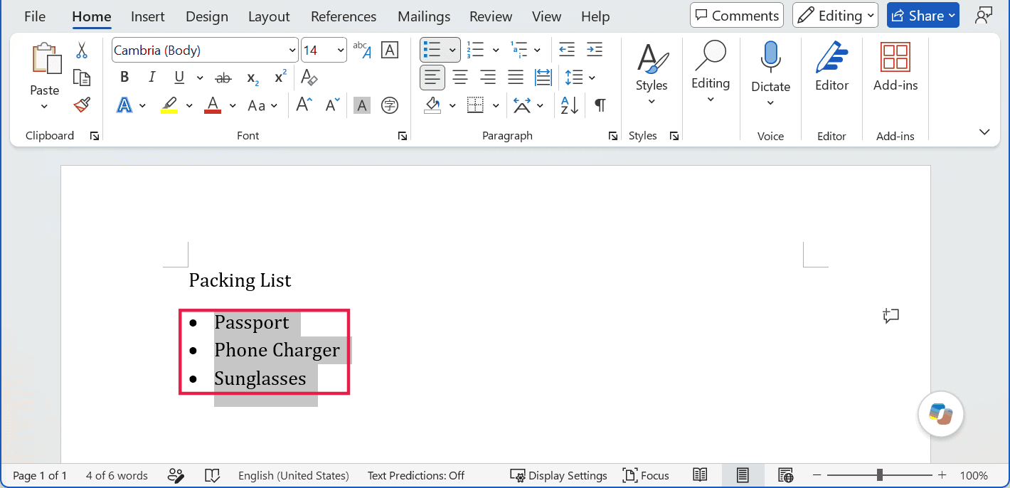
2. Double-click on the cell where you want to paste the list.

3. Press Control + V to paste it.

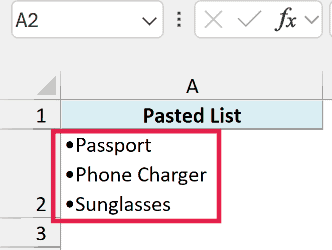
This will paste the bullet list in the same cell.

In this case, Word and PowerPoint behave differently. The list from Word gets pasted as is, while the one from PowerPoint gets pasted without the bullet points.

Copy bullet points into different cells

1. Copy the bullet points from Word or PowerPoint.

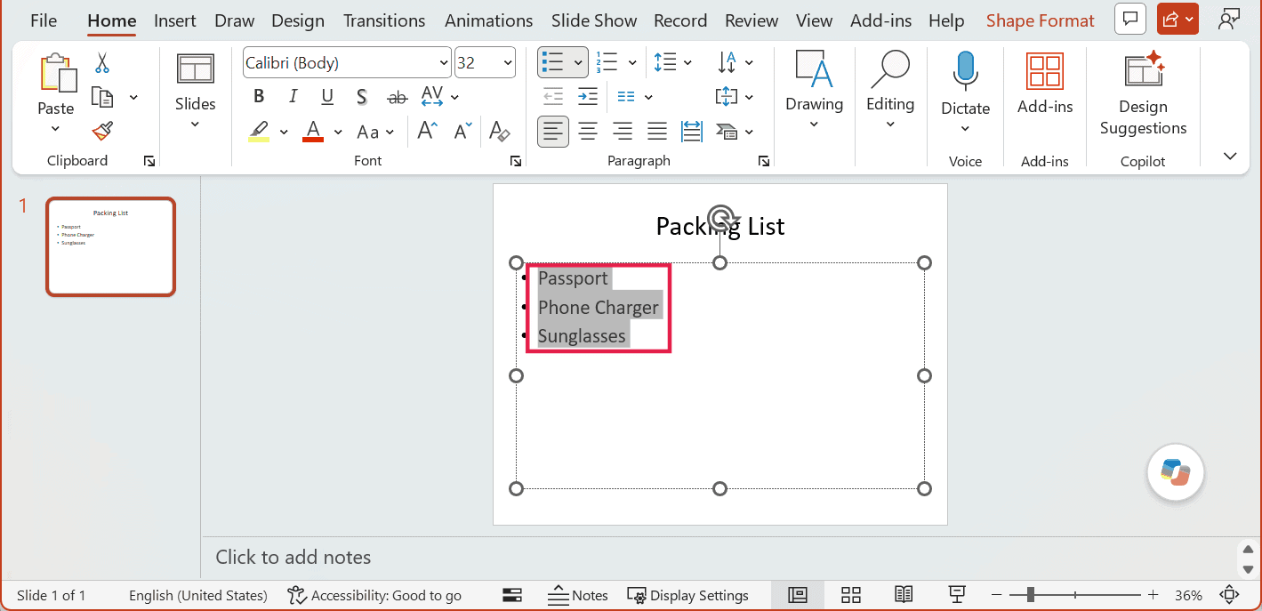
2. Select the cell where you want the list to start.

3. Press Control + V to paste it.

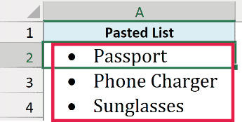
Each bullet point lands in its own cell.

Add Bullets in a Text Box or Shape

For a formatted list that floats over the sheet, such as a notes panel on a dashboard, a text box gives you bullets with indents.

This method puts the list in a text box, rather than inside a cell.

Here are the steps:

1. Go to the Insert tab > Text group > Text Box.

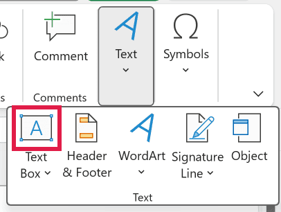
2. Draw the text box on the worksheet.

3. Type the items, pressing Enter after each one.

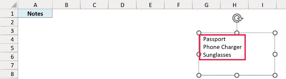
4. Select the text you want to turn into a bulleted list.

5. Right-click the selected text and choose Bullets.

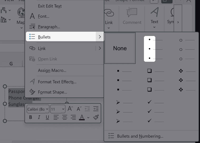
6. Pick a bullet style to apply it to your list.

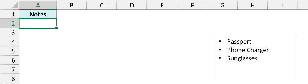
The same method works for text inside a shape.

These are eight simple ways you can use to add bullet points in Excel. Every method has its own benefits and can be used accordingly.

Hope you have enjoyed this article. Let me know your thoughts by leaving a comment below.

You May Also Like the Following Excel Tutorials:

• How to Insert Watermark in Excel Worksheets
• How to Type Degree Symbol in Excel
• How to Insert Delta Symbol in Excel
• How to Insert Line Break in Excel
• How to Insert Picture Into an Excel Cell
• How to Insert Rows in Excel
• How to Insert bullet points in Google Sheets