
Excel Custom Number formatting is the clothing for data in excel cells. You can dress these the way you want. All you need is a bit of know-how of how Excel Custom Number Format works.
With custom number formatting in Excel, you can change the way the values in the cells show up, but at the same time keeping the original value intact.
For example, I can make a date value show up in different Date formats, while the underlying value (the number that represents the date) would remain the same.
In this tutorial, I will cover everything about custom number format in Excel, and also show you some really useful examples that you can use in your day-to-day work.
So let’s get started!
Excel Custom Number Format Construct
Before I show you the awesomeness of it, let me briefly explain how custom number formatting works in Excel.
By design, Excel can accept the following four types of data in a cell:
- A positive number
- a negative number
- 0
- Text strings (this can include pure text strings as well as alphanumeric strings)
Another data type that Excel can accept is dates, but since all date and time values are stored as numbers in Excel, these would be covered as a part of the positive number.
For any cell in a worksheet in Excel, you can specify how each of these data types should be shown in the cell.
And below is the syntax in which you can specify this format.
<Format for POSITIVE Numer>;<Format for NEGATIVE Numer>;<Format for ZERO>;<Format for TEXT>
Note that all these are separated by semi-colons (;).
Anything that you enter in a cell in Excel would fall in either of these four categories and hence a custom format for it can be specified.
If you mention only:
- One format: It is applied to all four sections. For example, if you just write General, it will be applied for all four sections.
- Two formats: The first one is applied to positive numbers and zeros, and the second one is applied to negative numbers. Text format by default becomes General.
- Three Formats: The first one is applied to positive numbers, the second one is applied to negative numbers, the third is applied to zero, and the text disappears as nothing is specified for text.
If you want to learn more about custom number formatting, I would highly recommend the Office Help section.
How this works and where to enter these formats are covered later in this tutorial. For now, just keep in mind that this is the syntax for the format for any cell
How Custom Number Format Works in Excel
Then you open a new Excel workbook, by default all the cells in all the worksheets in that workbook have the General format where:
- Positive numbers are shown as is (aligned to the left)
- Negative numbers are shown with a minus sign (and aligned to the left)
- Zero is shown as 0 (and aligned to the left)
- Text is shown as is (aligned to the right)
And in case you enter a date, it’s shown based on your regional setting (in DD-MM-YYYY or MM-DD-YYYY format).
So by default, the cell’s number formatting is:
General;General;General;General
Where each data type is formatted as General (and follow the rules I mentioned above, based on whether it’s a positive number, negative number, 0, or text)
Now the default setting is alright, but how do you change the format. For example, if I want my negative numbers to show up in red color or I want my dates to show up in a specific format then how do I do that.
Using the Format Drop Down in the Ribbon
You can find some of the commonly used number formats in the Home tab within the Number group.
It’s a drop-down that shows many of the commonly used formats that you can apply to a cell by simply selecting the cell and then selecting the format from this list.

For example, if you want to convert numbers into percentages or converted dates into short date format or long-form date format, then you can easily do it by using the options in the dropdown.
Using Format Cells Dialog Box
Format cells dialog boxes where you get the maximum flexibility when it comes to applying formats to a cell in Excel.
It already has a lot of premade formats that you can use, or if you want to create your own custom number format, then you can do that as well.
Here is how to open the Format Cells dialog box;
- Click the Home Tab

- In the Number group, click on the dialog box launcher icon (the small tilted arrow at the bottom-right of the group).

This will open the Format Cells dialog box. Within it, you will find all the formats in the Number tab (along with the option to create Custom cell formats)
You can also use the following keyboard shortcut to open the format cells dialog box:
CONTROL + 1 (all the Control key and then press the 1 key).
In case you’re using Mac, you can use CMD + 1
Now let’s have a couple of practical examples where we will create our own custom number formats.
Also read: Cell References in Excel (Absolute, Relative, and Mixed)
Examples of Using Custom Number Formatting in Excel
Now let’s have a couple of practical examples where we will create our own custom number formats.
Hide a Cell Value (or Hide All values in a Range of Cells)
Sometimes, you may have a need to hide the content of the cell (without hiding the row or column that has the cell).
A practical case of this is when you are creating an Excel dashboard and there are a couple of values that you use in the dashboard but you do not want the users to see it. so you can simply hide these values
Suppose you have a dataset as shown below and you want to hide all the numeric values:

Here is how to do this using custom formatting in Excel:
- Select the cell or the range of cells for which you want to hide the cell content
- Open the Format Cells dialog box (keyboard shortcut Control + 1)
- In the Number tab, click on the Custom
- Enter the following format in the Type field:
;;;

How does this work?
The format for four different types of data types is divided by semicolons in the following format:
<Format for POSITIVE Numer>;<Format for NEGATIVE Numer>;<Format for ZERO>;<Format for TEXT>
In this technique, we have removed the format and only specified the semicolon, which indicates that we do not want any formatting for the cells. This is an indication for Excel to hide any content that is there in the cell.
Note that while this hides the content of the cell, it’s still there. so if you have numbers that you have hidden, you can still use these in calculations (which makes this a great trick for Excel dashboards and reports).
Display Negative Numbers in Red Color
By default, negative numbers show up with a minus sign (or within parenthesis in some regional settings).
You can use custom number formatting to change the color of the negative numbers and make them show up in red color.
Suppose you have a dataset as shown below and you want to highlight all the negative values in red color.

Below are the steps to do this:
- Select the range of cells where you want to show negative numbers in red
- Open the Format Cells dialog box (keyboard shortcut Control + 1)
- In the Number tab, click on the Custom
- Enter the following format in the Type field:
General;[Red]-General

The above format will make your cells with negative values show in red color.

How does this work?
When you only specify two formats as the custom number format, the first one is considered for positive numbers and 0, and the second one is considered for negative numbers (the next value by default becomes the general format).
In the above format that we have used, we have specified the color that we want that format to take up in the square brackets.
So while the negative numbers take the general format, they are shown in red color with a minus sign.
In case you want to make the negative numbers stop in red color within parenthesis (instead of the minus sign), you can use the below format:
General;[Red](General)

Also read: Show Negative Numbers in Parentheses (Brackets) in Excel (Easy Ways)
Add text to Numbers (such as Millions/Billions)
One amazing thing about custom number formatting is that you can add a prefix or a suffix text to a number, while still keeping the original number in the cell.
For example, I can have ‘100’ show up as ‘$100 Million’, while still having the original value in the cell so that I can use it in calculations.

Suppose you have a dataset as shown below and you want to show these numbers with a dollar sign and the word million in front of it.

Below are the steps to do this:
- Select the dataset where you want to add the text to the numbers
- Open the Format Cells dialog box (keyboard shortcut Control + 1)
- In the Number tab, click on the Custom
- Enter the following format in the Type field:
$General "Million"

Note that this custom number format will only affect numbers. If you enter text in the same cell, it would appear as it is.
How does this work?
In this example, to the general format, I have added the word million in double-quotes. anything that I add in double-quotes to the format is shown as is in the cell.
I also added the dollar sign before the general format so that all my numbers also show the dollar sign before the number.
Note: If you’re wondering why the dollar sign is not in double-quotes while the word Million is in double-quotes, it’s because Excel recognizes dollar as a symbol that is often used in custom number formatting, and doesn’t require you to add double quotes to it. You can go ahead and add double quotes to the dollar sign, but when you close the format cells dialog box and open it again, you will notice that Excel has removed it
Also read: Format Numbers to Show in Millions in Excel
Disguise Numbers and Text
With custom number formatting, you can assess a maximum of two conditions, and based on these conditions you can apply a format to the cell.
For example, suppose you have a list of scores for some students, you want to show the text Pass or Fail based on the score (where any score less than 35 should show ‘Fail’, else it should show ‘Pass’.

Below are the steps to show scores as Pass or Fail instead of the value using custom number format:
- Select the dataset where you have the scores
- Open the Format Cells dialog box (keyboard shortcut Control + 1)
- In the Number tab, click on the Custom
- Enter the following format in the Type field:
[<35]"Fail";"Pass"

Below is how your data would look after you have applied the above format.

Note that it does not change the value in the cells. The cell continues to have the scores in numeric values while displaying ‘Pass’ or ‘Fail’ depending on the cell value.
How does this work?
In this example, the condition needs to be specified within the square brackets. custom number formatting then evaluates the value in the cell and applies the format accordingly.
So if the value in the cell is less than 35, then the number is hidden, and instead the text ‘Fail’ is shown, adding all other cases, ‘Pass’ is shown.
Similarly, if you want to convert a range of cells that have 0’s and 1’s into TRUEs and FALSEs, you can use the below format:
[=0]"FALSE";[=1]"TRUE"
Remember that you can only use two conditions in custom number formatting. If you try and use more than two conditions, it is going to so your prompt letting you know that it cannot accept that format.
Hide Text but Display Numbers
Sometimes, when you download your data from databases since there are empty are filled with value such as Not Available or NA or –
With custom number formatting, you can hide all the text values while keeping the numbers as is. this also ensures that your original data is intact (as you are not deleting the text value, you’re just simply hiding it)
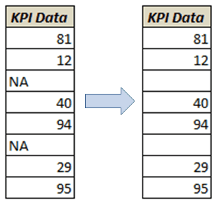
Suppose you have a data set as shown below where you want to hide all the text values:

Below are the steps to do this:
- Select the dataset where you have the data
- Open the Format Cells dialog box (keyboard shortcut Control + 1)
- In the Number tab, click on the Custom
- Enter the following format in the Type field:
General; -General; General;

Note that I have used the General format for numbers. You can any format you wish (such as 0, 0.#, #0.0%). Also, note that there is a negative sign (-) before the second General format, as it represents the format for negative numbers.
How does this work?
In this example, since we wanted to hide all the text values, we simply didn’t specify the format for it.
And since we specified the format for the other three data types (positive number, negative number, and zero), Excel understood that we have purposefully left the format for the text value empty, and it should not show anything if a cell has a text string.
Display Numbers as Percentages (%)
With custom number formatting, you can also change the numbers and make them show up in percentages.
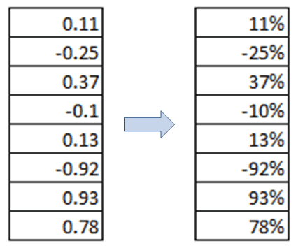
Suppose you have a data set as shown below, and you want to convert these numbers to show the equivalent percentage value:

Below are the steps to do this:
- Select the cells where you have the numbers (that you want to convert to percentage)
- Open the Format Cells dialog box (keyboard shortcut Control + 1)
- In the Number tab, click on the Custom
- Enter the following format in the Type field:
0%

This will change the numbers to their percentages. For example, it changes from 0.11 to 11%.
If all you want to do is converted a number into its equivalent percentage value, a better way to do this would be to use the percentage option in the format cells dialog box.
Where custom formatting can be useful is when you want more control over how you want to show the percentage value.
For example, if you want to show some additional text with the percentage, all you want to show negative percentages in red color then it is better to use custom formatting
Also read: How to Change Date Format In Excel?
Display Numbers in a Different Unit (Millions as Billions or Grams as Kilograms)
If you work with large numbers, you may want to show these in a different unit. for example, if you have the sales data of some companies, you may want to show the sales in millions or billions (while still keeping the original sale value in the cells)
Thankfully, you can easily do that with custom number formatting.
Suppose you have a data set as shown below, and you want to show these sales values in millions.

Below are the steps to do this:
- Select the cells where you have the numbers
- Open the Format Cells dialog box (keyboard shortcut Control + 1)
- In the Number tab, click on the Custom
- Enter the following format in the Type field:
0.0,,

The above would give you the result as shown below (values in millions in one digit after the decimal):

How does this work?
In the above format, a zero before the decimal indicates that Excel should show the entire number (exactly as it is in the cell), and a 0 after the decimal indicates that it should show only one significant digit after the decimal point.
So 0.0 would always be a number with one digit after the decimal point.
When you add a comma after the 0.0, it will shave off the last three-digit of the number. For example, 123456 would become 123.4 (the last three digits are removed, and since it has to show 1 digit after the decimal point, it shows 4)
If you think about it, it’s similar to dividing the number by 1000. So if you want to show a number in the ‘millions’ unit, you need to add 2 commas, so that it would shave off the last 6 digits.
And if you also want to show the word million or the alphabet M after the number, use the below format
0.0,, "M"
You May Also Like the Following Excel Tutorials:
- Disguise Numbers as Text in a Drop Down List in Excel.
- Color Negative Chart Data Labels in Red with a downward arrow.
- How to Copy Conditional Formatting to Another Cell in Excel
- How to Remove Cell Formatting in Excel (from All, Blank, Specific Cells)
- How to Remove Table Formatting in Excel
- How To Convert Date To Serial Number In Excel?
- Change the Default Font in Excel
- How to Format Phone Numbers in Excel?


I hope you can still answer.
How would you format a custom cell that includes both numbers and characters, e.g., 12345abcd678e9 to 12345-abc-d78-e9
Hello Francisco… You can’t do this using Custom Number formatting. It can only allow you to specify the format for Positive numbers, Negative numbers, zero and text. The text you mentioned would be considered text value (as it’s alphanumeric). With custom formatting, you can show 12345abcd678e9 as is or specify what else you want to show instead of this. What you’re trying to achieve can be done using formulas (if there is a consistent pattern that can be followed)
Sir, 7th May,2020.
Very nicely and clearly you have shown every item.So, understanding clearly.
thanking you and expect to receive such useful notes in future too.
Once again Thanking you.
Kanhaiyalal Newaskar.
I have been following your excel module guide and it has taught me a lot of things I was missing out on in Excel.
These shortcuts are very well explained, extremely helpful, and time saving.
Thank you.
I am really happy to read all your article. You did a Amazing JOB!!! Very Appreciate!!!!!BIG BLESS~~~
Excellent!
Except ;;;; should be ;;; surely?
Thanks for letting me know. Yes, it should have been three semi-colons only. Have corrected it
Hi, thank for the tips, but once we’ve created the format we want, is there a way to create a shortcut to the new custom number format?
I can’t find a way that answers what you’re probably after, Manu, but if you select a cell that has the formatting you want, and press Ctrl+1 it will take you straight to that format.
Which, now I think about it, is a useful way to check what format a cell (or range of cells) is. If the range of cells comes up with no format (not even “General”), then you have a mixture of formats in that range.