
Since dates and times are stored as numbers in the back end in Excel, you can easily use simple arithmetic operations and formulas on the date and time values.
For example, you can add two different time values or date values or you can calculate the time difference between two given dates/times.
In this tutorial, I will show you a couple of ways to perform calculations using time in Excel (such as calculating the time difference, adding or subtracting time, showing time in different formats, and doing a sum of time values)
How Excel Handles Date and Time?
As I mentioned, dates and times are stored as numbers in a cell in Excel. A whole number represents a complete day and the decimal part of a number would represent the part of the day (which can be converted into hours, minutes, and seconds values)
For example, the value 1 represents 01 Jan 1900 in Excel, which is the starting point from which Excel starts considering the dates.
So, 2 would mean 02 Jan 1990, 3 would mean 03 Jan 1900 and so on, and 44197 would mean 01 Jan 2021.
Note: Excel for Windows and Excel for Mac follow different starting dates. 1 in Excel for Windows would mean 1 Jan 1900, and 1 in Excel for Mac would mean 1 Jan 1904
If there are any digits after a decimal point in these numbers, Excel would consider those as part of the day and it can be converted into hours, minutes, and seconds.
For example, 44197.5 would mean 01 Jan 2021 12:00:00 PM.

So if you’re working with time values in Excel, you would essentially be working with the decimal portion of a number.
And Excel gives you the flexibility to convert that decimal portion into different formats such as hours only, minutes only, seconds only, or a combination of hours, minutes, and seconds
Now that you understand how time is stored in Excel, let’s have a look at some examples of how to calculate the time difference between two different dates or times in Excel
Formulas to Calculating Time Difference Between Two Times
In many cases, all you want to do is find out the total time that has elapsed between the two-time values (such as in the case of a timesheet that has the In-time and the Out-time).
The method you choose would depend on how the time is mentioned in a cell and in what format you want the result.
Let’s have a look at a couple of examples
Simple Subtraction of Calculate Time Difference in Excel
Since time is stored as a number in Excel, find the difference between 2 time values, you can easily subtract the start time from the end time.
End Time – Start Time
The result of the subtraction would also be a decimal value that would represent the time that has elapsed between the two time-values.
Below is an example where I have the start and the end time and I have calculated the time difference with a simple subtraction.

There is a possibility that your results are shown in the time format (instead of decimals or in hours/minutes values). In our above example, the result in cell C2 shows 09:30 AM instead of 9.5.
That’s perfectly fine as Excel tries to copy the format from the adjacent column.
To convert this into a decimal, change the format of the cells to General (the option is in the Home tab in the Numbers group)
Once you have the result, you can format it in different ways. For example, you can show the value in hours only or minutes only or a combination of hours, minutes, and seconds.
Below are the different formats you can use:
| Format | What it Does |
| h | Shows only the hours elapsed between the two dates |
| hh | Shows hours in double-digit (such as 04 or 12) |
| hh:mm | Shows hours and minutes elapsed between the two dates, such as 10:20 |
| hh:mm:ss | Shows hours, minutes, and seconds elapsed between the two dates, such as 10:20:36 |
And if you’re wondering where and how to apply these custom date formats, follow the below steps:
- Select the cells where you want to apply the date format
- Hold the Control key and press the 1 key (or Command + 1 if using Mac)
- In the Format Cells dialog box that opens, click on the Number tab (if not selected already)

- In the left pane, click on Custom

- Enter any of the desired format code in the Type field (in this example, I am using hh:mm:ss)

- Click OK
The above steps would change the formatting and show you the value based on the format.

Note that custom number formatting does not change the value in the cell. It only changes the way a value is being displayed. So, I can choose to only show the hour value in a cell, while it would still have the original value.
Pro tip: If the total number of hours exceeds 24 hours, use the following custom number format instead: [hh]:mm:ss
Calculate the Time Difference in Hours, Minutes, or Seconds
When you subtract the time values, Excel returns a decimal number that represents the resulting time difference.
Since every whole number represents one day, the decimal part of the number would represent that much part of the day which can easily be converted into hours or minutes, or seconds.
Calculating Time Difference in Hours
Suppose you have the dataset as shown below and you want to calculate the number of hours between the two-time values

Below is the formula that will give you the time difference in hours:
=(B2-A2)*24
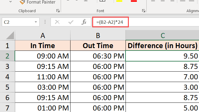
The above formula will give you the total number of hours elapsed between the two-time values.
Sometimes, Excel tries to be helpful and will give you the result in time format as well (as shown below).

You can easily convert this into Number format by clicking on the Home tab, and in the Number group, selecting Number as the format.

If you only want to return the total number of hours elapsed between the two times (without any decimal part), use the below formula:
=INT((B2-A2)*24)

Note: This formula only works when both the time values are of the same day. If the day changes (where one of the time values is of another date and the second one of another date), This formula will give wrong results. Have a look at the section where I cover the formula to calculate the time difference when the date changes later in this tutorial.
Calculating Time Difference in Minutes
To calculate the time difference in minutes, you need to multiply the resulting value by the total number of minutes in a day (which is 1440 or 24*60).
Suppose you have a data set as shown below and you want to calculate the total number of minutes elapsed between the start and the end date.
Below is the formula that will do that:
=(B2-A2)*24*60

Calculating Time Difference in Seconds
To calculate the time difference in seconds, you need to multiply the resulting value by the total number of seconds in a day (which is or 24*60*60 or 86400).
Suppose you have a data set as shown below and you want to calculate the total number of seconds that have elapsed between the start and end date.
Below is the formula that will do that:
=(B2-A2)*24*60*60

Calculating time difference with the TEXT function
Another easy way to quickly get the time difference without worrying about changing the format is to use the TEXT function.
The TEXT function allows you to specify the format right within the formula.
=TEXT(End Date - Start Date, Format)
The first argument is the calculation you want to do, and the second argument is the format in which you want to show the result of the calculation.
Suppose you have a dataset as shown below and you want to calculate the time difference between the two times.
Here are some formulas that will give you the result with different formats
Show only the number of hours:
=TEXT(B2-A2,"hh")

The above formula will only give you the result that shows the numbers of hours elapsed between the two-time values. If your result is 9 hours and 30 minutes, it will still show you 9 only.
Show the number of total minutes
=TEXT(B2-A2,"[mm]")

Show the number of total seconds
=TEXT(B2-A2,"[ss]")

Show Hours and Minutes
=TEXT(B2-A2,"[hh]:mm")

Show Hours, Minutes, and Seconds
=TEXT(B2-A2,"hh:mm:ss")

If you’re wondering what’s the difference between hh and [hh] in the format (or mm and [mm]), when you use the square brackets, it would give you the total number of hours between the two dates, even if the hour value is higher than 24. So if you subtract two date values where the difference is more than24 hours, using [hh] will give you the total number of hours and hh will only give you the hours elapsed on the day of the end date.
Get the Time Difference in One-Unit (Hours/Minutes) and Ignore Others
If you want to calculate the time difference between the two time-values in only the number of hours or minutes or seconds, then you can use the dedicated HOUR, MINUTE, or SECOND function.
Each of these functions takes one single argument, which is the time value, and returns the specified time unit.
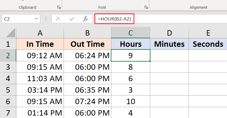
Suppose you have a data set as shown below, and you want to calculate the total number of hours minutes, and seconds that have elapsed between these two times.

Below are the formulas to do this:
Calculating Hours Elapsed Between two times
=HOUR(B2-A2)
Calculating Minutes from the time value result (excluding the completed hours)
=MINUTE(B2-A2)

Calculating Seconds from the time value result (excluding the completed hours and minutes)
=SECOND(B2-A2)

A couple of things that you need to know when working with these HOURS, MINUTE, and SECOND formulas:
- The difference between the end time and the start time cannot be negative (which is often the case when the date changes). In such cases, these formulas would return a #NUM! error
- These formulas only use the time portion of the resulting time value (and ignore the day portion). So if the difference in the end time and the start time is 2 Days, 10 Hours, 32 Minutes, and 44 Seconds, the HOUR formula will give 10, the MINUTE formula will give 32, and the SECOND formula will give 44
Calculate elapsed time Till Now (from the start time)
If you want to calculate the total time that has elapsed between the start time and the current time, you can use the NOW formula instead of the End time.
NOW function returns the current date and the time in the cell in which it is used. It’s one of those functions that does not take any input argument.
So, if you want to calculate the total time that has elapsed between the start time and the current time, you can use the below formula:
=NOW() - Start Time
Below is an example where I have the start times in column A, and the time elapsed till now in column B.

If the difference in time between the start date and time and the current time is more than 24 hours, then you can format the result to show the day as well as the time portion.
You can do that by using the below TEXT formula:
=TEXT(NOW()-A2,"dd hh:ss:mm")
You can also achieve the same thing by changing the custom formatting of the cell (as covered earlier in this tutorial) so that it shows the day as well as the time portion.
In case your start time only has the time portion, then Excel would consider it as the time on 1st January 1990.
In this case, if you use the NOW function to calculate the time elapsed till now, it is going to give you the wrong result (as the resulting value would also have the total days that have elapsed since 1st Jan 1990).
In such a case, you can use the below formula:
=NOW()- INT(NOW())-A2
The above formula uses the INT function to remove the day portion from the value returned by the now function, and this is then used to calculate the time difference.
Note that NOW is a volatile function that updates whenever there is a change in the worksheet, but it does not update in real-time
Calculate Time When Date Changes (calculate and display negative times in Excel)
The methods covered so far work well if your end time is later than the start time.
But the problem arises when your end time is lower than the start time. This often happens when you are filling timesheets where you only enter the time and not the entire date and time.
In such cases, if you’re working in a one night shift and the date changes, there is a possibility that your end time would be earlier than your start time.
For example, if you start your work at 6:00 PM in the evening, and complete your work & time out at 9:00 AM in the morning.
If you only working with time values, then subtracting the start time from the end time is going to give you a negative value of 9 hours (9 – 18).
And Excel cannot handle negative time values (and for that matter nor can humans, unless you can time travel)
In such cases, you need a way to figure out that the day has changed and the calculation should be done accordingly.
Thankfully, there is a really easy fix for this.
Suppose you have a dataset as shown below, where I have the start time and the end time.

As you would notice that sometimes the start time is in the evening and the end time is in the morning (which indicates that this was an overnight shift and the day has changed).
If I use the below formula to calculate the time difference, it will show me the hash signs in the cells where the result is a negative value (highlighted in yellow in the below image).
=B2-A2

Here is an IF formula that whether the time difference value is negative or not, and in case it is negative then it returns the right result
=IF((B2-A2)<0,1-(A2-B2),(B2-A2))

While this works well in most cases, it still falls short in case the start time and the end time is more than 24 hours apart. For example, someone signs in at 9:00 AM on day 1 and sign-out at 11:00 AM on day 2.
Since this is more than 24 hours, there is no way to know whether the person has signed out after 2 hours or after 26 hours.
While the best way to tackle this would be to make sure that the entries include the date as well as the time, but if it’s just the time that you’re working with, then the above formula should take care of most of the issues (considering it’s unlikely for anyone to work for more than 24 hours)
Adding/ Subtracting Time in Excel
So far, we have seen examples where we had the start and the end time, and we needed to find the time difference.
Excel also allows you to easily add or subtract a fixed time value from the existing date and time value.
For example, let’s say you have a list of queued tasks where each task takes the specified time, and you want to know when each task will end.
In such a case, you can easily add the time that each task is going to take to the start time to know at what time is the task expected to be completed.
Since Excel stores date and time values as numbers, you have to ensure that the time you are trying to add abides by the format that Excel already follows.
For example, if you add 1 to a date in Excel, it is going to give you the next date. This is because 1 represents an entire day in Excel (which is equal to 24 hours).
So if you want to add 1 hour to an existing time value, you cannot go ahead and simply add 1 to it. you have to make sure that you convert that hour value into the decimal portion that represents one hour. and the same goes for adding minutes and seconds.
Using the TIME Function
Time function in Excel takes the hour value, the minute value, and the seconds value and converts it into a decimal number that represents this time.
For example, if I want to add 4 hours to an existing time, I can use the below formula:
=Start Time + TIME(4,0,0)

This is useful if you know how many hours, minutes, and seconds you want to add to an existing time and simply use the TIME function without worrying about the correct conversion of the time into a decimal value.
Also, note that the TIME function will only consider the integer part of the hour, minute, and seconds value that you input. For example, if I use 5.5 hours in the TIME function it would only add five hours and ignore the decimal part.
Also, note that the TIME function can only add values that are less than 24 hours. If your hour value is more than 24, this would give you an incorrect result.
And the same goes with the minutes and the second’s part where the function will only consider values that are less than 60 minutes and 60 seconds
Just like I have added time using the TIME function, you can also subtract time. Just change the + sign to a negative sign in the above formulas
Using Basic Arithmetic
When the time function is easy and convenient to use, it does come with a few restrictions (as covered above).
If you want more control, you can use the arithmetic method that I’ll cover here.
The concept is simple – convert the time value into a decimal value that represents the portion of the day, and then you can add it to any time value in Excel.
For example, if you want to add 24 hours to an existing time value, you can use the below formula:
=Start_time + 24/24
This just means that I’m adding one day to the existing time value.
Now taking the same concept forward let’s say you want to add 30 hours to a time value, you can use the below formula:
=Start_time + 30/24
The above formula does the same thing, where the integer part of the (30/24) would represent the total number of days in the time that you want to add, and the decimal part would represent the hours/minutes/seconds
Similarly, if you have a specific number of minutes that you want to add to a time value then you can use the below formula:
=Start_time + (Minutes to Add)/24*60
And if you have the number of seconds that you want to add, then you can use the below formula:
=Start_time + (Minutes to Add)/24*60*60
While this method is not as easy as using the time function, I find it a lot better because it works in all situations and follows the same concept. unlike the time function, you don’t have to worry about whether the time that you want to add is less than 24 hours or more than 24 hours
You can follow the same concept while subtracting time as well. Just change the + to a negative sign in the formulas above
How to SUM time in Excel
Sometimes you may want to quickly add up all the time values in Excel. Adding multiple time values in Excel is quite straightforward (all it takes is a simple SUM formula)
But there are a few things you need to know when you add time in Excel, specifically the cell format that is going to show you the result.
Let’s have a look at an example.
Below I have a list of tasks along with the time each task will take in column B, and I want to quickly add these times and know the total time it is going to take for all these tasks.

In cell B9, I have used a simple SUM formula to calculate the total time all these tasks are going to take, and it gives me the value as 18:30 (which means that it is going to take 18 hours and 20 minutes to complete all these tasks)

All good so far!
How to SUM over 24 hours in Excel
Now see what happens when I change at the time it is going to take Task 2 to complete from 1 hour to 10 hours.

The result now says 03:20, which means that it should take 3 hours and 20 minutes to complete all these tasks.
This is incorrect (obviously)
The problem here is not Excel messing up. The problem here is that the cell is formatted in such a way that it will only show you the time portion of the resulting value.
And since the resulting value here is more than 24 hours, Excel decided to convert the 24 hours part into a day remove it from the value that is shown to the user, and only display the remaining hours, minutes, and seconds.
This, thankfully, has an easy fix.
All you need to do is change the cell format to force it to show hours even if it exceeds 24 hours.
Below are some formats that you can use:
| Format | Expected Result |
| [h]:mm | 28:30 |
| [m]:ss | 1710:00 |
| d “D” hh:mm | 1 D 04:30 |
| d “D” hh “Min” ss “Sec” | 1 D 04 Min 00 Sec |
| d “Day” hh “Minute” ss “Seconds” | 1 Day 04 Minute 00 Seconds |
You can change the format by going to the format cells dialog box and applying the custom format, or use the TEXT function and use any of the above formats in the formula itself
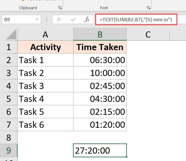
You can use the below the TEXT formula to show the time, even when it’s more than 24 hours:
=TEXT(SUM(B2:B7),"[h]:mm:ss")
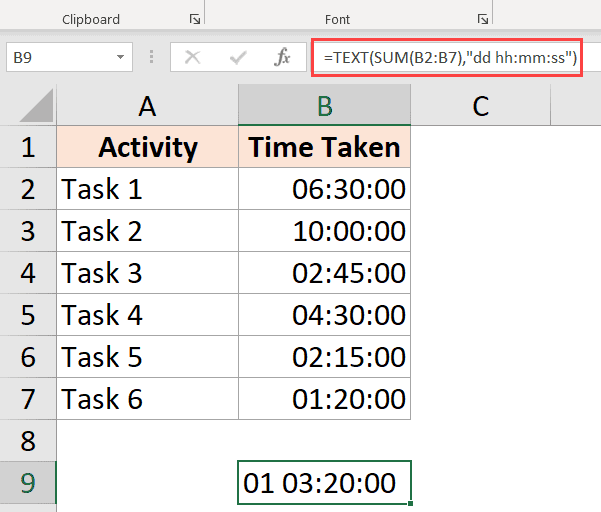
or the below formula if you want to convert the hours exceeding 24 hours to days:
=TEXT(SUM(B2:B7),"dd hh:mm:ss")
Results Showing Hash (###) Instead of Date/Time (Reasons + Fix)
In some cases, you may find that instead of showing you the time value, Excel is displaying the hash symbols in the cell.
Here are some possible reasons and the ways to fix these:
The column is not wide enough
When a cell doesn’t have enough space to show the complete date, it may show the hash symbols.
It has an easy fix – change the column width and make it wider.
Negative Date Value
A date or time value cannot be negative in Excel. in case you are calculating the time difference and it turns out to be negative, Excel will show you hash symbols.
The way to fixes to change the formula to give you the right result. For example, if you are calculating the time difference between the two times, and the date changes, you need to adjust the formula to account for it.
In other cases, you may use the ABS function to convert the negative time value into a positive number so that it’s displayed correctly. Alternatively, you can also an IF formula to check if the result is a negative value and return something more meaningful.
In this tutorial, I covered topics about calculating time in Excel (where you can calculate the time difference, add or subtract time, show time in different formats, and sum time values)
I hope you found this tutorial useful.
Other Excel tutorials you may also like:
- Convert Time to Decimal Number in Excel (Hours, Minutes, Seconds)
- How to Remove Time from Date/Timestamp in Excel
- How to Calculate the Number of Days Between Two Dates in Excel
- Combine Date and Time in Excel
- How to Calculate Years of Service in Excel
- How to Convert Seconds to Minutes in Excel
- Convert Minutes to Hundredths in Excel


