Combine Date and Time in Excel (3 Easy Ways)

Sometimes you may have dates in one column and time values in another column and you want to combine these to get one single date and time value in a cell.

And if you’re thinking that you can do that by easily combining the two cells by using the concatenate formula or the & sign, you’ll find out that it doesn’t work.

I have tried to use the & sign to combine the cells that contain date and time, and the resulting value is not in the expected format.

In this tutorial, I will show you three ways to quickly combine date and time values in Excel, two with formulas and one with Power Query.

So let’s get started!

Combine Date and Time in One Cell with a Simple Addition

Excel stores date and time values as numbers in the back end.

For example, 44197.375 in Excel represents 01-01-2021 09:00 AM.

The integer part of the above number represents a date (which is 01 Jan 2021), and the decimal part of the number represents a time (which is 9 AM).

So, if you have dates in one column and time in another column, the easiest way to combine these and get the date and time in one single cell would be to simply add these two cells.

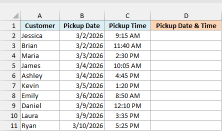
Below is a list of store pickups with the pickup date and the pickup time in separate columns, and I want the combined date and time in column D.

Below is the formula that will do that:

=B2:B11+C2:C11

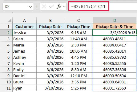
This formula adds each date in column B to the time next to it in column C. Since it’s a dynamic array formula, you enter it once in D2 and the results spill down to D11 automatically.

As I mentioned, dates and times are stored as numbers in Excel. The combined date and time values that you see in column D are also decimal numbers in the back end.

This is why the formatting matters here. When you enter this formula, Excel gives D2 a date and time format on its own, but the cells the result spills into stay in the General format.

So D2 shows 3/2/2026 9:15 (with US date settings), while the cells below it show numbers like 46083.48611.

To fix this, change the cell formatting of the whole column using the Format Cells dialog box (where you can specify the custom code to show the date and time in a specific way).

Here are the steps to do this:

1. Select the cells that have the result (D2:D11 in our example).

2. Press Ctrl + 1 (Command + 1 on a Mac) to open the Format Cells dialog box.

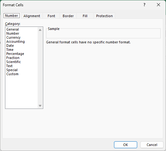
3. In the Number tab, click Custom in the Category list.

4. In the Type field, enter m/d/yyyy h:mm AM/PM.

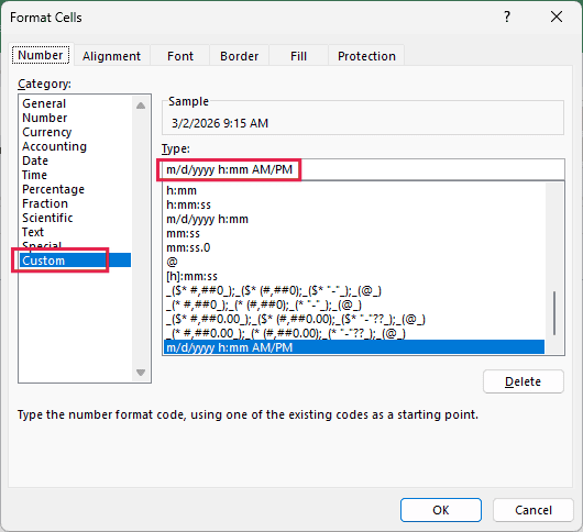
5. Click OK.

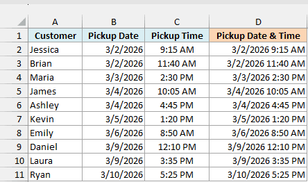
Now every cell in column D shows the date as well as the time, such as 3/2/2026 9:15 AM.

If you see ### in some cells, the column isn’t wide enough for the full date and time. Double-click the right edge of the column header to widen it.

Pro Tip: You can use any other date and time code in the Type field. For example, dd-mmm-yyyy hh:mm shows 02-Mar-2026 09:15, and the value in the cell stays exactly the same.

If you are using Excel 2019 or earlier, enter the below formula in cell D2 and then copy it down to all the cells in the column:

=B2+C2

It gives the same result, and when you copy the formula down, the date and time format from D2 gets copied along with it.

Concatenate Date and Time Using the TEXT Function

Another quick way to combine date and time in Excel is by using the TEXT function to join them as text.

If you join a date cell and a time cell directly with the & sign, you get the numbers Excel stores in the back end, something like 46083 0.385416666666667. The TEXT function fixes this by converting each value into text in the format you specify.

Below is the same list of store pickups, and I want the date and time joined together as text in column D.

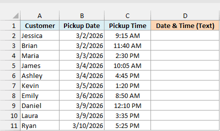
Below is the formula that can do this:

=TEXT(B2:B11,"dd-mmm-yyyy")&" "&TEXT(C2:C11,"hh:mm AM/PM")

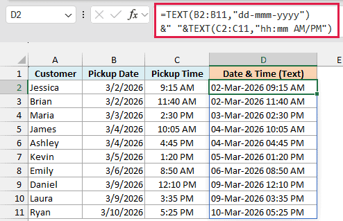
The TEXT function allows you to take any value as the input and show it in the specified format.

In our example, I have used two TEXT functions. The first one takes the date value and displays it as a date (02-Mar-2026), and the second one takes the time value and displays it as the time (09:15 AM).

If your time values have seconds, use “hh:mm:ss AM/PM” as the time format so the seconds show up too.

And since I want both of these in the same cell, I have used the & sign to join them, with a space as the separator in between the date and time. The results spill down to D11 automatically.

Since we have used the TEXT function to specify the format for the date and the time, it does not matter how the input values are displayed in the cell.

For example, even if I have the numerical values instead of the date and the time, this formula would still give me the right result.

Important: The result of this formula is a text string, not a real date and time value. You can’t use it in date calculations, and sorting puts 04-Mar-2026 04:45 PM ahead of 04-Mar-2026 10:05 AM, so use the addition method when you need a real value.

You can also get the same result with a single TEXT function by adding the date and time first:

=TEXT(B2:B11+C2:C11,"dd-mmm-yyyy hh:mm AM/PM")

It’s shorter, but the two-TEXT version lets you format the date and the time separately.

If you prefer the CONCAT function, the below formula gives the same result. Enter it in cell D2 and copy it down, because CONCAT joins everything you give it into one cell and can’t spill a separate result for each row:

=CONCAT(TEXT(B2,"dd-mmm-yyyy")," ",TEXT(C2,"hh:mm AM/PM"))

The below formula does the same thing with the & sign and works in every version of Excel, including Excel 2019 or earlier. Enter it in cell D2 and then copy it down:

=TEXT(B2,"dd-mmm-yyyy")&" "&TEXT(C2,"hh:mm AM/PM")

Another big benefit of using the TEXT function is that you can combine other text strings with the result of this formula.

To give you an example, let’s say I don’t want just the date and the time. I want the result in the following format: Date: 02 Mar 2026, Time: 09:15 AM.

To do this, you can use the below formula:

="Date: "&TEXT(B2:B11,"dd mmm yyyy")&", Time: "&TEXT(C2:C11,"hh:mm AM/PM")

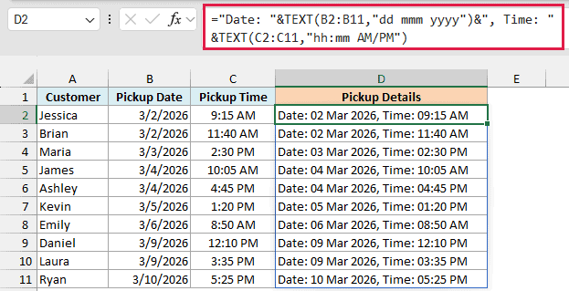
Since the result of the TEXT function is a text string, we can easily combine it with the other text strings using the ampersand operator (&) or the CONCAT function.

Merge Date and Time Columns Using Power Query

If you get this kind of data regularly (say, a weekly export from another system), Power Query can combine the date and time columns for you. You set up the steps once and refresh whenever the data changes.

Below is the same list of store pickups in an Excel Table named Pickups, and I want a combined date and time column in a new table next to it.

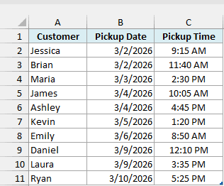
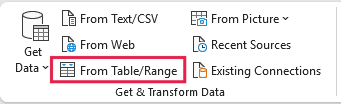
Power Query works from an Excel Table. If your data is a plain range, Excel offers to convert it into a table when you click From Table/Range.

Here are the steps:

1. Select any cell in the Pickups table.

2. Click the Data tab.

3. In the Get & Transform Data group, click From Table/Range.

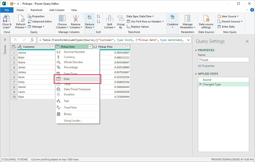
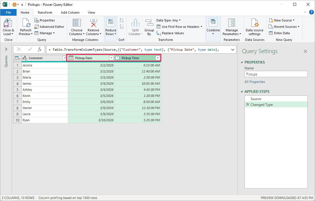
This opens the Power Query editor. Power Query reads the pickup dates as Date/Time values and the pickup times as decimal numbers.

Combine Date and Time joins a Date column with a Time column, so you need to change both columns to the right data type first.

4. Click the data type icon at the left of the Pickup Date column header and select Date.

5. In the Change Column Type dialog box, click Replace current.

6. Click the data type icon at the left of the Pickup Time column header and select Time.

7. In the Change Column Type dialog box, click Replace current.

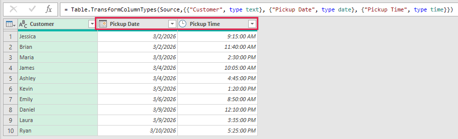
8. Click the Pickup Date column header.

9. Hold the Ctrl key and click the Pickup Time column header.

10. Click the Add Column tab.

11. In the From Date & Time group, click Date.

12. Select Combine Date and Time.

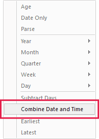
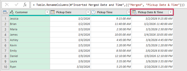
Power Query adds a new column named Merged at the end, with each row’s date and time combined into a single value.

13. Double-click the Merged column header, type Pickup Date & Time, and press Enter.

14. Click the Home tab.

15. Click the Close & Load drop-down arrow and select Close & Load To.

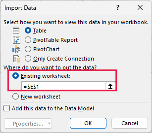
16. In the Import Data dialog box, select Existing worksheet.

17. In the box below it, enter =$E$1.

18. Click OK.

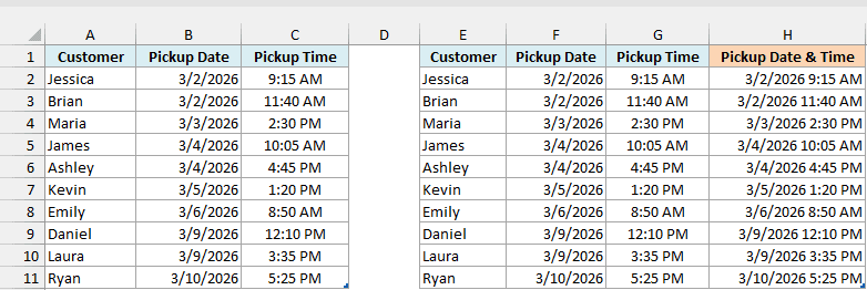
This places the result table next to the source table, starting in cell E1, so both tables are visible. If you click Close & Load instead, Excel puts the result on a new worksheet.

The best part about this method is that the result stays connected to the Pickups table. When you add new pickups or change existing ones, right-click any cell in the result table and choose Refresh, and Power Query runs the same steps again.

So these are three simple ways you can use to combine date and time in Excel.

I hope you found this tutorial useful.

Other Excel tutorials you may also like:

• Calculate Time in Excel (Time Difference, Hours Worked, Add/ Subtract)
• Convert Time to Decimal Number in Excel (Hours, Minutes, Seconds)
• How to Remove Time from Date/Timestamp in Excel
• How to Quickly Insert Date and Timestamp in Excel
• How to Change Date Format In Excel?
• How to Add Months to Date in Excel
• How to Compare Dates in Excel (Greater/Less Than, Mismatches)
• TIME Function in Excel
• DATE Function in Excel
• NOW Function in Excel