
If you work with a lot of numbers in Excel, it’s a good practice to highlight negative numbers in red. This makes it easier to read the data.
There are various techniques you can use to highlight negative numbers in red in Excel:
- Using Conditional Formatting
- Using Inbuilt Number Formatting
- Using Custom Number Formatting
Let’s explore each of these techniques in detail.
Highlight Negative Numbers in Red – Using Conditional Formatting
Excel Conditional formatting rules are applied to a cell based on the value it holds.
In this case, we will check whether the value in a cell in less than 0 or not. If it is, then the cell can be highlighted in a specified color (which would be red in this case).
Here are the steps to do this:
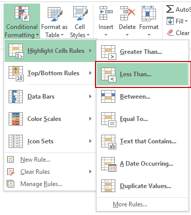
- Go to Home → Conditional Formatting → Highlight Cell Rules → Less Than.
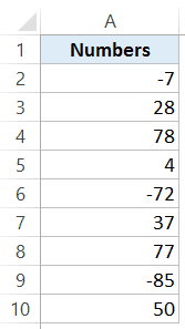
- Select the cells in which you want to highlight the negative numbers in red.
- In the Less Than dialog box, specify the value below which the formatting should be applied. If you want to use formatting other than the ones in the drop-down, use the Custom Format option.
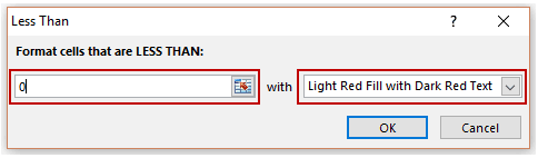
- Click OK.
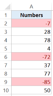
All the cells with a value less than 0 would get highlighted in Light Red color with dark red text in it.
Using conditional formatting is also helpful when you want to print the reports. While you may not see a significant difference in the font color in a black and white printout, since conditional formatting highlights the entire cell, it makes the highlighted cells stand out.
Caution: Conditional Formatting is volatile, which means that it recalculates whenever there is a change in the workbook. While the impact is negligible on small data sets, you may see some drag because of it when applied to large datasets.
Highlight Negative Numbers in Red – Using Inbuilt Excel Number Formatting
Excel has some inbuilt number formats that make it super easy to make negative numbers red in Excel.
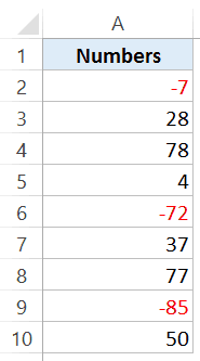
When you apply the ‘Number’ format, it adds two decimals to the numbers and makes the negative numbers show up in red.
Something as shown below:

To do this:
- Select the cells in which you want to highlight the negative numbers in red.
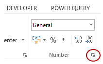
- Go to the Home tab → Number Format group and click on the dialog launcher (it is the small tilted arrow icon at the bottom right of the group. This will open the Format Cell dialog box (or you can use the keyboard shortcut Control + 1).
- In the Format Cells dialog box, within the Number tab, select Number in the Category list. In the option on the right, select the red text in the ‘Negative numbers’ options.
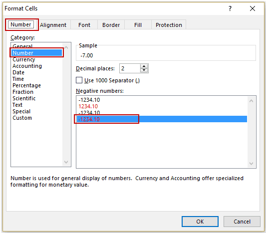
- Click OK.
This would automatically add two decimal points and make the negative numbers red with a minus sign.
Note that none of the techniques shown in this tutorial change the value in the cell. It only changes the way the value is displayed.
Also read: Show Negative Numbers in Parentheses (Brackets) in Excel
Highlight Negative Numbers in Red – Using Custom Number Formats
If the inbuilt formats are not what you want. Excel allows you to create your own custom formats.
Here are the steps:
- Select the cells in which you want to highlight the negative numbers in red.
- Go to the Home tab → Number Format group and click on the dialog launcher. This will open the Format Cell dialog box (or you can use the keyboard shortcut Control + 1).
- In the Number tab, select Custom from the Category list and use the below format in type: General;[Red]-General
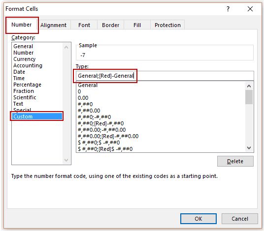
- Click OK.
This will make the negative numbers show up in red, while everything else remains the same.
How this works:
There are four format types that you can customize in Excel:
<Positive Numbers>;<Negative Numbers>;<Zeroes>;<Text>
These formats are separated by a semicolon.
You can specify the format for each type and it will show up that way in Excel.
For using colors, you can specify the color in square brackets at the beginning of the format. Not all colors are supported in custom number formatting, but you can use common colors such as red, blue, green, yellow, cyan, etc.
You can specify a format for any or all of these four parts. For example, if you write General;General;General;General then everything is in the General format.
But if you write 0.00;-0.00;0.00;General, positive numbers are displayed with 2 decimals, negative with a negative sign and 2 decimals, zero as 0.00, and text as normal text.
Similarly, you can specify the format for any of the four parts.
If you mention only:
- One format: It is applied to all the four sections. For example, if you just write General, it will be applied for all the four sections.
- Two formats: The first one is applied to positive numbers and zeros, and the second is applied to negative numbers. Text format by default becomes General.
- Three Formats: The first one is applied to positive numbers, the second is applied to negative numbers, the third is applied to zero, and the text disappears as nothing is specified for text.
If you want to learn all about custom number formatting, I would highly recommend Office Help section.
You May Also Like the Following Excel Tutorials:


PERFECT
THIS IS GREAT FOR A BEGINNER LIKE ME SELF TEACHING
How we can show highlighted 0 in red in excel pivot charts?
I can’t figure out how to do this when it is pulling the data into the cell from another tab. The formatting doesn’t seem to apply
check this
http://tutorialway.com/microsoft-excel-font-formatting/
I have a formatting problem that you might be able to help me with. My objective is to have a comma format with floating decimal. #,###,### almost gets the result I want except whole numbers are displayed with a decimal. For example, “1001.001” appears as “1,001.001”, exactly as I want it, but “1001” appears as “1,001.” (includes decimal point) when I want it to appear as “1,001” (no decimal point). Other than using VBA to test and format each entry or a conditional format for every cell in the workbook, I cannot seem to find a solution. Any ideas?
Hello Jim, As far as I know, there is no way to get floating decimal using custom number formatting or any other non-VBA method
using number format and currecncy format colour is not getting changed. Do i need to set something else?
Hey.. You need to open the format cells dialog box and then select the number format (with red text). I have updated the tutorial to show the steps.
got it. tks