
A few days ago, I was working on creating an Excel dashboard.
I had to create a number of drop-downs with the options ranging from 1 to 5. To make it more user-friendly, I also wanted to give an option of ‘Not Selected’, when a user does not want to make a selection in the drop down list in Excel.
Something as shown below in the pic:
The problem here is that when I choose ‘Not Selected’ from the drop down, it returns the text Not Selected (see in the formula bar in the pic above). Since I have to use this selection in some formulas, I want this to return a 0.
Now there are 2 ways to format numbers as text using Number Custom Formatting.
Method 1: Format Numbers as Text in Drop Down List in Excel
You can format numbers as text in the drop down list in Excel in such a way, that it shows text in the drop down, but when selected, gets stored as a number in the cell.
Here are the steps to do this:
- In a cell type 0 (this is the cell that you want to be displayed as ‘Not Selected’).
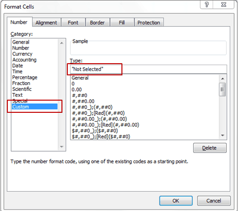
- With the cell selected, press Control + 1 (this opens the Format Cells dialogue box).
- Select the Number tab and go to Custom option.
- In Custom, type “Not Selected” as shown in the pic.
- That’s it!! Now you will have a cell that has Not Selected in it, but in the formula bar displays a 0. When I use this in creating a drop down list, a user can select the option ‘Not Selected’ and this would return 0 (as shown below in the pic).

Also read: Convert Text to Number in Excel
Method 2 – Format Number as Text in the Cell in Excel
While the above trick works fine, in terms of creating dashboards, it makes more sense to display ‘Not Selected’ in the drop down menu as well as in the cell (when it is selected), instead of a 0 (as shown in the pic below; notice the value in formula bar). This makes it easier for someone else to pick-up the spreadsheet and works on it.

Again, this can be done very easily using custom formats.
Here are 2 quick ways to do this:
- Select the cell that has the drop down validation list and press Control + 1 (This opens the Format Cells dialogue box).
- Select the Number tab and go to Custom option.
- Type [=0]”Not Selected” OR Type 0;0;”Not Selected”.
- Click OK.
How it works
Custom Number Formatting has for components (separated by semi-colon):
<Positive Numbers> ; <Negative Numbers> ; <Zero> ; <Text>
These four parts can be formatted separately to give the desired format.
For example, in the case above, we wanted to display 0 as Not Selected. In the number formatting sequence, 0 is the third part of the format, so we changed the sequence to 0;0;”Not Selected”.
This means that positive and negative numbers are displayed as it is, and whenever there is a zero, it is displayed as Not Selected.
The other way is to give a condition to number format [=0]”Not Selected”. This display Not Selected whenever the value in a cell is 0, else it will use the General formatting settings.
Here are a couple of good sources to learn more about Custom Number Formatting:
Other Excel articles you may also like:


What if I want my drop down to show only text, but represent numbers, for example: (drop down shows) always, sometimes, never. Numeric value is 3, 2, 1 (respectively). But I would like it to display always, sometimes, never….but I want to quantify it with an average score at the end. Is there a way to do that using your awesome simple method?