How to Remove Leading Zeros in Excel (5 Easy Ways)

Many people have a love-hate relationship with leading zeros in Excel.

Sometimes you want it, and sometimes you don’t.

While Excel has been programmed in such a way that it automatically removes any leading zeros from the numbers, there are some cases when you may have these.

In this Excel tutorial, I will show you how to remove the leading zeros in your numbers in Excel.

So let’s get started!

Possible Reasons You May Have Leading Zeros in Excel

As I mentioned, Excel automatically removes any leading zeros from numbers. For example, if you enter 00100 in a cell in Excel, it would automatically convert it into 100.

In most cases, this makes sense as these leading zeros are not really meaningful.

But in some cases, you may want it.

Here are some possible reasons that may cause your numbers to retain the leading zeros:

• If the number has been formatted as text (mostly by adding an apostrophe before the number), it would retain the leading zeros.
• The cell may have been formatted in such a way that it always shows a certain length of a number. And in case the number is smaller, leading zeros are added to make up for it. For example, you can format a cell to always show 5 digits (and if the number is less then five digits, leading zeros are added automatically)

The method we choose to remove the leading zeros would depend on what is causing it.

Also read: How to Add Leading Zeroes in Excel

So, the first step is to identify the cause so that we can choose the right method to remove these leading zeros.

How to Remove Leading Zeros from Numbers

There are multiple ways you can use to remove the leading zeros from numbers.

In this section, I will show you five such methods.

Convert the Text to Numbers Using the Error Checking Option

If the cause of leading numbers is that someone has added apostrophe before these numbers (to convert these into text), you can use the error checking method to convert these back into numbers with a single click.

This is probably the easiest method to get rid of leading zeros.

Here I have a data set where I have the numbers that have an apostrophe before these as well as the leading zeros. This is also the reason you see these numbers aligned to the left (whereas by default numbers align to the right) and also have the leading 0’s.

Below are the steps to remove these leading zeros from these numbers:

1. Select the numbers from which you want to remove the leading zeros. You will notice that there is a yellow icon at the top right part of the selection.
2. Click on the yellow error checking icon
3. Click on ‘Convert to Number’

That’s it! The above steps would remove the apostrophe and convert these text values back into numbers.

And since Excel is programmed to remove leading spaces from any numbers by default, you’ll see that doing this automatically removes all the leading zeros.

Change the Custom Number Formatting of the Cells

Another really common reason that may make your numbers show up with leading zeros is when your cells have been formatted to always show a specific number of digits in each number.

A lot of people want to make the numbers look consistent and of the same length, so they specify the minimum length of the numbers by changing the formatting of the cells.

For example, if you want all the numbers to show up as 5 digits numbers, if you have a number which is only three-digit Excel would automatically add two leading zeros to it.

Below I have a dataset where custom number formatting has been applied to always show a minimum of five digits in the cell.

And the way to get rid of these leading zeros is just to remove the existing formatting from the cells.

Below are the steps to do this:

1. Select the cells that have the numbers with the leading zeros
2. Click the Home tab
3. In the Numbers group, click on the Number Format dropdown
4. Select ‘General’

The above steps would change the custom number formatting of the cells and now the numbers would be displayed as expected (where there would be no leading zeros).

Note that this technique would only work when the reason for the leading zeroes was custom number formatting. It would not work if an apostrophe has been used to convert numbers to text (in which case you should use the previous method)

Multiply by 1 (using Paste Special technique)

This technique works in both scenarios (where the numbers have been converted into text by using an apostrophe or a custom number formatting has been applied to the cells).

Suppose you have a data set as shown below and you want to remove the leading zeros from it.

Below are the steps to do this

1. Copy any empty cell from the worksheet
2. Select the cells where you have the numbers from which you want to remove the leading zeros
3. Right-click on the selection and then click on Paste Special. This will open the Paste Special dialog box
4. Click on the ‘Add’ option (in the operations group)
5. Click OK

The above steps add 0 to the range of cells you selected and also remove all the leading zeros and apostrophe.

While this does not change the value of the cell, it converts all the text values into numbers as well as copies the formatting from the blank cell that you copied (thereby replacing the existing formatting that was making the leading zeros show up).

This method only impacts the numbers. In case you have any text string in a cell, it would remain unchanged.

Using the VALUE function

Another quick and easy method to remove the leading zeros is to use the value function.

This function takes one argument (which could be the text or the cell reference that has the text) and returns the numerical value.

This would also work in both scenarios where your leading numbers are a result of the apostrophe (used to convert numbers to text) or the custom number formatting.

Suppose I have a data set as shown below:

Below is the formula that would remove the leading zeros:

=VALUE(A1)

Using Text to Columns

While the Text to Columns functionality is used to split a cell into multiple columns, you can also use it to remove the leading zeros.

Suppose you have a data set as shown below:

Below are the steps to remove leading zeros using Text to Columns:

1. Select the range of cells that have the numbers
2. Click on the ‘Data’ tab
3. In the Data Tools group, click on ‘Text to Columns’
4. In the ‘Convert Text to Columns’ wizard, make the following changes:
   1. Step 1 of 3: Select ‘Delimited’and click on Next
   2. Step 2 of 3: Deselect all the delimiters and click on Next
   3. Step 3 of 3: Select a destination cell (B2 in this case) and click on Finish

The above steps should remove all the leading zeros and give you only the numbers. In case you still see the leading zeros, you need to change the formatting of the cells to General (this can be done from the Home tab)

How to Remove Leading Zeros from Text

While all the above methods work great, these are meant for only those cells that have a numerical value.

But what if you have alphanumeric or text values that also happened to have some leading zeros in it.

The above methods would not work in that case, but thanks to amazing formulas in Excel, you can still get this time.

Suppose you have a data set as shown below and you want to remove all the leading zeros from it:

Below is the formula to do that:

=RIGHT(A2,LEN(A2)-FIND(LEFT(SUBSTITUTE(A2,"0",""),1),A2)+1)

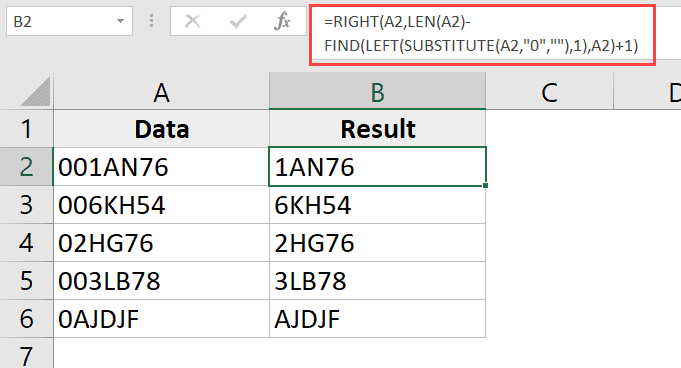
Let me explain how this formula works

The SUBSTITUTE part of the formula replaces the zero with a blank. So for the value 001AN76, the substitute formula gives the result as 1AN76

The LEFT formula then extracts the left-most character of this resulting string, which would be 1 in this case.

The FIND formula then looks for this left-most character given by the LEFT formula and returns its position. In our example, for the value 001AN76, it would give 3 (which is the position of 1 in the original text string).

1 is added to the result of the FIND formula, to make sure that we get the entire text string extracted (except the leading zeros)

The result of the FIND formula is then subtracted from the result of the LEN formula (which is used to give the length of the entire text string). This gives us the length of the text ring without the leading zeros.

This value is then used with the RIGHT function to extract the entire text string (except the leading zeros).

In case there is a possibility that there may be leading or trailing spaces in your cells, it’s best to use the TRIM function with every cell reference.

So the new formula with the TRIM function added would be as shown below:

=RIGHT(TRIM(A2),LEN(TRIM(A2))-FIND(LEFT(SUBSTITUTE(TRIM(A2),"0",""),1),TRIM(A2))+1)

So, these are some easy ways that you can use to remove leading zeros from your data set in Excel.

I hope you found this tutorial useful!

Other Excel tutorials you may like:

• Hide Zero Values in Excel | Make Cells Blank If the Value is 0
• How to Replace Blank Cells with Zeros in Excel Pivot Tables
• Delete Rows Based on a Cell Value (or Condition) in Excel
• How to Stop Excel from Changing Numbers to Dates
• How to Convert Serial Numbers to Dates in Excel