Hide Zero Values in Excel | Make Cells Blank If the Value is 0

Watch Video – How to Hide Zero Values in Excel + How to Remove Zero Values

In case you prefer reading over watching a video, below is the complete written tutorial.

Sometimes in Excel, you may want to hide zero values in your dataset and show these cells as blanks.

Suppose you have a dataset as shown below and you want to hide the value 0 in all these cells (or want to replace it with something such as a dash or the text ‘Not Available’).

While you can do this manually with a small dataset, you’ll need better ways when working with large datasets.

In this tutorial, I will show you multiple ways to hide zero values in Excel and one method to select and remove all the zero values from the dataset.

Let’s get started and dive into each of these methods!

Automatically Hide Zero Value in Cells

Excel has an inbuilt functionality that allows you to automatically hide all the zero values for the entire worksheet.

All you have to do is uncheck a box in Excel options, and the change will be applied to the entire worksheet.

Suppose you have the sales dataset as shown below and you want to hide all the zero values and show a blank cells instead.

Below are the steps to hide zeros from all the cells in a workbook in Excel:

1. Open the workbook in which you want to hide all the zeros
2. Click the File tab
3. Click on Options
4. In the Excel Options dialog box that opens, click on the ‘Advanced’ option in the left pane
5. Scroll down to the section that says ‘Display option for this worksheet’, and select the worksheet in which you want to hide the zeros.
6. Uncheck the ‘Show a zero in cells that have zero value’ option
7. Click Ok

The above steps would instantly hide zeros in all the cells in the selected worksheet.

This change is also applied to cells where zero is a result of a formula.

Remember that this method only hides the 0 value in the cells and doesn’t remove these. The 0 is still there, it’s just hidden.

Hide Zero Value in Cells using Conditional Formatting

While the above method is the most convenient one, it doesn’t allow you to hide zeros only in a specific range (rather it hides zero values in the entire worksheet).

In case you only want to hide zeros for a specific dataset (or multiple datasets), you can use conditional formatting.

With conditional formatting, you can apply a specific format based on the value in the cells. So, if the value in some cells is 0, you can simply program conditional formatting to hide it (or even highlight it if you want).

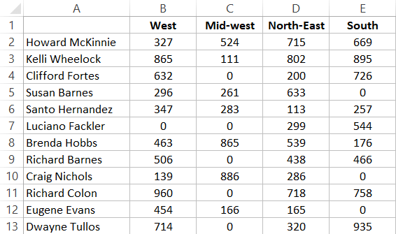
Suppose you have a dataset as shown below and you want to hide zeros in the cells.

Below are the steps to hide zeros in Excel using conditional formatting:

1. Select the dataset
2. Click the ‘Home’ tab
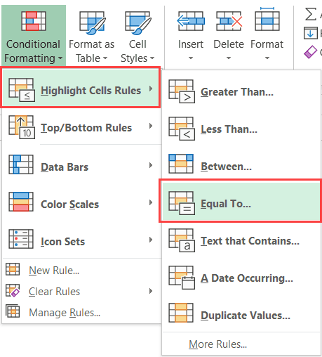
3. In the ‘Styles’ group, click on ‘Conditional Formatting’.
4. Place the cursor over the ‘Highlight Cells Rules’ options and in the options that show up, click on the ‘Equal to’ option.
5. In the ‘Equal To’ dialog box, enter ‘0’ in the left field.
6. Select the Format drop-down and click on ‘Custom Format’.
7. In the ‘Format Cells’ dialog box, select the ‘Font’ tab.
8. From the Color drop-down, choose the white color.
9. Click OK.
10. Click OK.

The above steps change the font color of the cells that have the zeros to white, which make these cells look blank.

This workaround works only when you have a white background in your worksheet. In case there is any other background-color in the cells, the white color may still keep the zeros visible.

In case you want to truly hide the zeros in the cells, where the cells look blank no matter what background color is given to the cells, you can use the steps below.

1. Select the dataset
2. Click the ‘Home’ tab
3. In the ‘Styles’ group, click on ‘Conditional Formatting’.
4. Place the cursor over the ‘Highlight Cells Rules’ options and in the options that show up, click on the ‘Equal to’ option.
5. In the ‘Equal To’ dialog box, enter 0 in the left field.
6. Select the Format drop-down and click on Custom Format.
7. In the ‘Format Cells’ dialog box, select the ‘Number’ tab and click on the ‘Custom’ option in the left pane.
8. In the Custom format option, enter the following in the Type field: ;;; (three semi-colons without space)
9. Click OK.
10. Click OK.

The above steps change the custom formatting of cells that have the value 0.

When you use three semi-colons as the format, it hides everything in the cell (be it numeric or text). And since this format is applied only to those cells which have the value 0 in it, it only hides the zeros and not the rest of the dataset.

Both the methods covered above also work when 0 is a result of a formula in a cell.

Hide Zero Value using Custom Formatting

Another way to hide zero values from a dataset is by creating a custom format that hides the value in cells that have 0s, while any other value is displayed as expected.

Below are the steps to use a custom format to hide zeros in cells:

1. Select the entire dataset for which you want to apply this format. If you want this for the entire worksheet, select all the cells
2. With the cells selected, click the Home tab
3. In the Cells group, click the Format option
4. From the drop-down option, click on Format Cells. This will open the Format cells dialog box
5. In the Format Cells dialog box, select the Number tab
6. In the option on the left pane, click on the Custom option.
7. In the options on the right, enter the following format in the Type field: 0;-0;;@
8. Click OK

The above steps would apply a custom format to the selected cells where only those cells which have the value 0 are formatted to hide the value, while the rest of the cells display the data as expected.

How does this custom format work?

In Excel, there are four types of data formats that you specify:

1. Positive numbers
2. Negative numbers
3. Zeros
4. Text

And for each of these data types, you can specify a format.

In most cases, there is a default format – General, which keeps all these data types visible. But you have the flexibility of creating a specific format for each of these data types.

Below is the custom format structure you need to follow in case you are applying a custom format to each of these data types:

<Positive Numbers>;<Negative Numbers>;<Zeros>;<Text>

In the method covered above, I have specified the format to:

0;-0;;@

The above format does the following:

1. Positive numbers are shown as is
2. Negative numbers are shown with a negative sign
3. Zeros are hidden (as no format is specified)
4. Text is shown as is

Replace Zeros with Dash or Some Specific Text

In some cases, you may want to not just hide the zeros in the cells, but replace these with something more meaning.

For example, you may want to remove the zeros and replace it with a dash or a text such as “Not Available” or “Data Yet to Come”

This is again made possible using custom number formatting, where you can specify what a cell should display instead of a zero.

Below are the steps to convert a 0 to a dash in Excel:

1. Select the entire dataset for which you want to apply this format. If you want this for the entire worksheet, select all the cells
2. With the cells selected, click the Home tab
3. In the Cells group, click the Format option
4. From the drop-down option, click on Format Cells. This will open the Format cells dialog box
5. In the Format Cells dialog box, select the Number tab
6. In the option on the left pane, click on the Custom option.
7. In the options on the right, enter the following format in the Type field: 0;-0;–;@
8. Click OK

The above steps would keep all the other cells as is and change the cells with the value 0 to show a dash (–).

Hide Zero Values in Pivot Tables

There can be two scenarios where a Pivot Table shows the value as 0:

1. The source data cells that are summarized in the Pivot Table has 0 values
2. The source data cells that are summarized in the Pivot Table are blanks and the Pivot table has been formatted to show the empty cells as zero

Let’s see how to hide the zeros in the Pivot table in each scenario:

When Source Data cells have 0s

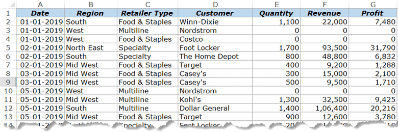
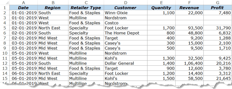
Below is a sample dataset that I have used to create a Pivot table. Note that the Quantity/Revenue/Profit numbers for all the records for ‘West’ are 0.

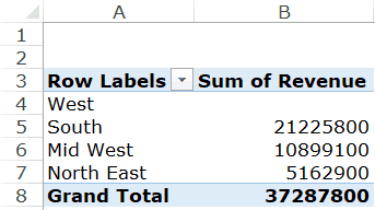
The Pivot table created using this data set looks as shown below:

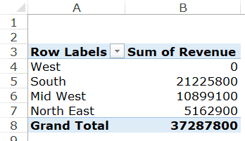
Since there were 0s in the dataset for all the records for West region, you see a 0 in the Pivot table for west here.

If you want to hide zero in this Pivot Table, you can use conditional formatting to do this.

However, conditional formatting in the Pivot Table in Excel works a little different than regular data.

Here are the steps to apply conditional formatting to Pivot Table to hide zeros:

1. Select any cell in the column that has 0s in the Pivot Table summary (Do not select all the cells, but only one cell)
2. Click the Home tab
3. In the ‘Styles’ group, click on ‘Conditional Formatting’.
4. Place the cursor over the ‘Highlight Cells Rules’ options and in the options that show up, click on the ‘Equal to’ option.
5. In the ‘Equal To’ dialog box, enter 0 in the left field.
6. Select the Format drop-down and click on Custom Format.
7. In the ‘Format Cells’ dialog box, select the Number tab and click on the ‘Custom’ option in the left pane.
8. In the Custom format option, enter the following in the Type field: ;;; (three semi-colons without space)
9. Click OK. You will see small Formatting Options icon at the right of the selected cell.
10. Click on this ‘Formatting Options’ icon
11. In the options that become available, choose – All cells showing “Sum of Revenue” values for “Region”.

The above steps hide the zero in the Pivot Table in such a way that if you change the Pivot Table structure (by adding more rows/columns headers to it, the zeros will continue to be hidden).

If you want to learn more about how this works, here is a detailed tutorial on the right way to apply conditional formatting to Pivot Tables.

When Source Data cells have empty cells

Below is an example where I have a dataset that has empty cells for all the records for West.

If I create a Pivot Table using this data, I will get the result as shown below.

By default, the Pivot Table shows you empty cells when all the cells in the source data are blank. But in case you still see a 0 in this case, follow the below steps to hide the zero and show blank cells:

1. Right-click on any of the cells in the Pivot Table
2. Click on ‘Pivot Table Options’
3. In the ‘PivotTable Options’ dialog box, click on the ‘Layout & Format’ tab
4. In the Format options, check the options and ‘For empty cells show:’ and leave it blank.
5. Click OK.

The above steps would hide the zeros in the Pivot Table and show a blank cell instead.

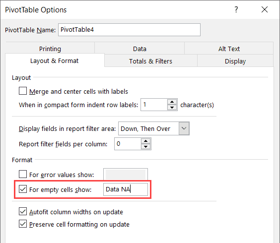
In case you want the Pivot Table to show something instead of the 0, you can specify that in step 4. For example, if you want to show the text – ‘Data not Available’, instead of the 0, type this text in the field (as shown below).

Find and Remove Zeros in Excel

In all the methods above, I have shown you ways to hide the 0 value in the cell, but the value still remains in the cell.

In case you want to remove the zero values from the dataset (which would leave you with blank cells), use the below steps:

1. Select the dataset (or the entire worksheet)
2. Click the Home tab
3. In the ‘Editing’ group, click on ‘Find & Select’
4. In the options that are shown in the drop-down, click on ‘Replace’
5. In the ‘Find and Replace’ dialog box, make the following changes:
   • In the ‘Find what’ field, enter 0
   • In the ‘Replace with’ field, enter nothing (leave it empty)
   • Click on Options button and check the ‘Match entire cell contents’ option
6. Click on Replace All

The above steps would instantly replace all the cells that had zero value with a blank.

In case you don’t want to remove the zeros right away and first select the cells, use the following steps:

1. Select the dataset (or the entire worksheet)
2. Click the Home tab
3. In the ‘Editing’ group, click on ‘Find & Select’
4. In the options that are shown in the drop-down, click on ‘Replace’
5. In the ‘Find and Replace’ dialog box, make the following changes:
   • In the ‘Find what’ field, enter 0
   • In the ‘Replace with’ field, enter nothing (leave it empty)
   • Click on Options button and check the ‘Match entire cell contents’ option
6. Click on the ‘Find All’ button. This will give you a list of all the cells that have 0 in it
7. Press Control-A (hold the control key and press A). This will select all the cells that have 0 in it.

Now, that you have all the cells with 0 selected, you can delete these, replace these with something else, or change the color and highlight these.

Hiding the Zeros Vs. Removing The Zeros

When treating the cells with 0s in it, you need to know the difference between hiding these and removing these.

When you hide the zero value in a cell, it is not visible to you, but it still remains in the cell. This means that if you have a dataset and you use it for calculation, that 0 value will also be used in the calculation.

On the contrary, when you have a blank cell, using it in formulas may mean that Excel automatically ignores these cells (depending on which formula you’re using).

For example, below is what I get when I use the AVERAGE formula to get the average for two columns (the result is in row 14). Column A has cells where the 0 value has been hidden (but is still there in the cell) and Column B has cells where the 0 value has been removed.

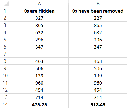
You can see the difference in the result despite the fact that the dataset for both datasets looks the same.

This happens as the AVERAGE formula ignores blank cells in column B, but it uses the ones in Column A (as the ones in column A still has the value 0 in it).

You may also like the following Excel tutorials:

• How to Hide a Worksheet in Excel
• Delete Rows Based on a Cell Value
• Delete Blank Rows in Excel
• How to Delete Every Other Row in Excel (or Every Nth Row)
• Show Formulas in Excel Instead of the Values
• Change Negative Number to Positive in Excel
• How to Remove Leading Zeros in Excel