How to Find Circular Reference in Excel (Quick and Easy)

While working with Excel formulas, you may sometime see the following warning prompt.

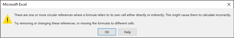
This prompt tells you that there is a circular reference in your worksheet and this can lead or an incorrect calculation by the formulas. It also asks you to address this circular reference issue and sort it.

In this tutorial, I will cover all that you need to know about circular reference, and well as how to find and remove circular references in Excel.

So let’s get started!

What is Circular Reference in Excel?

In simple words, a circular reference happens when you end up having a formula in a cell – which in itself uses the cell (in which it’s been entered) for the calculation.

Let me try and explain this by a simple example.

Suppose you have the dataset in cell A1:A5 and you use the below formula in cell A6:

=SUM(A1:A6)

This will give you a circular reference warning.

This is because you want to sum the values in cell A1:A6, and the result should be in cell A6.

This creates a loop as Excel just keeps on adding the new value in cell A6, which keeps on changing (hence, a circular reference loop).

How to Find Circular References in Excel?

While the circular reference warning prompt is kind enough to tell you that it exists in your worksheet, it doesn’t tell you where it’s happening and what cell references are causing it.

So if you’re trying to find and handle circular references in the worksheet, you need to know a way to somehow find these.

Below are the steps to find a circular reference in Excel:

1. Activate the worksheet that has the circular reference
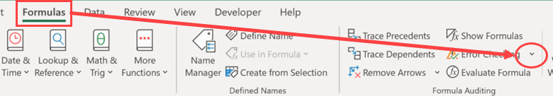
2. Click the Formulas tab
3. In the Formula Editing group, click on the Error Checking drop-down icon (little downward pointing arrow at the right)
4. Hover the cursor over the Circular References option. It will show you the cell that has a circular reference in the worksheet
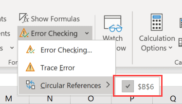
5. Click on the cell address (that is displayed) and it will take you to that cell in the worksheet.

Once you have addressed the issue, you can again follow the same steps above and it will show more cell references that have the circular reference. If there is none, you will not see any cell reference,

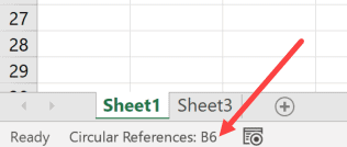
Another quick and easy way to find the circular reference is by looking at the Status bar. On the left part of it, it will show you the text Circular Reference along with the cell address.

There are a few things you need to know when working with circular references:

1. In case the iterative calculation is enabled (covered later in this tutorial), the status bar will not show the circular reference cell address
2. In case the circular reference is not in the active sheet (but in other sheets in the same workbook), it will only show Circular reference and not the cell address
3. In case you get a circular reference warning prompt once and you dismiss it, it will not show the prompt again the next time.
4. If you open a workbook that has the circular reference, it will show you the prompt as soon as the workbook opens.

How to Remove a Circular Reference in Excel?

Once you have identified that there are circular references in your sheet, it’s time to remove these (unless you want them to be there for a reason).

Unfortunately, it’s not as simple as hitting the delete key. Since these are dependent on formulas and every formula is different, you need to analyze this on a case-by-case basis.

In case it’s just a matter of having the cell reference causing the issue by mistake, you can simply correct by adjusting the reference.

But sometimes, it’s not that simple.

Circular reference can also be caused based on multiple cells that feed into each other at many levels.

Let me show you an example.

Below there is a circular reference in cell C6, but it’s not just a simple case of self-reference. It’s multi-level where the cells it uses in the calculations also reference each other.

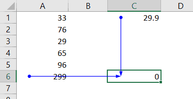
• The formulas in cell A6 is =SUM(A1:A5)+C6
• The formula is cell C1 is =A6*0.1
• The formula in cell C6 is =A6+C1

In the above example, the result in cell C6 is dependent on the values in cell A6 and C1, which in turn are dependent on cell C6 (thus causing the circular reference error)

And again, I have chosen a really simple example just for demo purposes. In reality, these could be quite difficult to figure out and maybe far off in the same worksheet or even scattered across multiple worksheets.

In such a case, there is one way to identify the cells that are causing circular reference and then treat these.

It’s by using the Trace Precedents option.

Below are the steps to use trace precedents to find cells that are feeding to the cell that has the circular reference:

1. Select the cell that has the circular reference
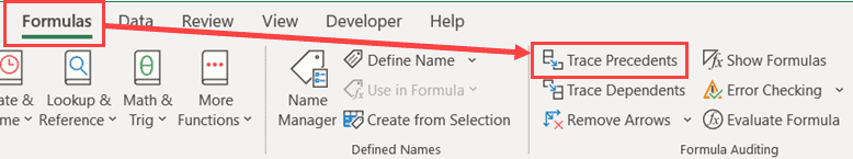
2. Click the Formulas tab
3. Click on Trace Precedents

The above steps would show you blue arrows which will tell you what cells are feeding into the formula in the selected cell. This way, you can inspect the formulas and the cells and get rid of the circular reference.

In case you’re working with complex financial models, it may be possible that these precedents also go multiple levels deep.

This works well if you have all the formulas referring to cells in the same worksheet. If it’s in multiple worksheets, this method is not effective.

How to Enable/Disable Iterative Calculations in Excel

When you have a circular reference in a cell, first you get the warning prompt as shown below, and if you close this dialog box, it will give you 0 as the result in the cell.

This is because when there is a circular reference, it’s an endless loop and Excel doesn’t want to caught up in it. So it returns a 0.

But in some cases, you may actually want the circular reference to be active and do a couple of iterations. In such a case, instead of an infinite loop, and you can decide how many times the loop should be run.

This is called iterative calculation in Excel.

Below are the steps to enable and configure iterative calculations in Excel:

1. Click the File tab
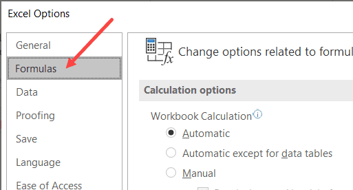
2. Click on Options. This will open the Excel Options dialog box
3. Select Formula in the left pane
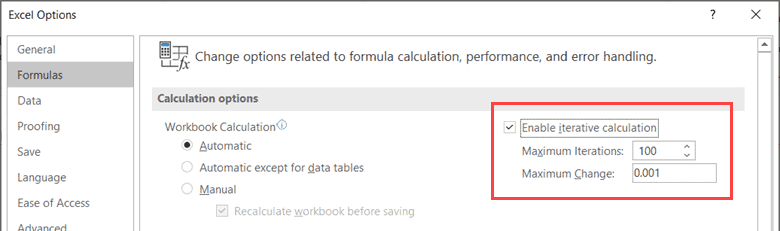
4. In the Calculation options section, check the box ‘Enable iterative calculation’. Here you can specify the maximum iterations and maximum change value

That’s it! The above steps would enable iterative calculation in Excel.

Let me also quickly explain the two options in the iterative calculation:

• Maximum iterations: This is the maximum number of times you want Excel to calculate before giving you the final result. So if you specify this as 100, Excel will run the loop 100 times before giving you the final result.
• Maximum Change: This is the maximum change, which if not achieved between iterations, the calculation would be stopped. By default, the value is .001. The lower this value, the more accurate would be the result.

Remember that the more number of times the iterations run, the more time and resources it takes for Excel to do it. In case you keep the maximum iterations high, it may lead to your Excel slowing down or crashing.

Deliberately Using Circular References

In most cases, the presence of circular reference in your worksheet would be an error. And this is why Excel shows you a prompt which says – “Try removing or changing these references or moving the formulas to different cells.”

But there might be some specific cases where you need a circular reference so that you can get the desired result.

One such specific case I have already written about it getting the time stamp in a cell in a cell in Excel.

For example, suppose you want to create a formula so that every an entry is made in a cell in Column A, the timestamp appear in Column B (as shown below):

While you can insert easily insert a timestamp using the below  formula:

=IF(A2<>"",IF(B2<>"",B2,NOW()),"")

The issue with the above formula is that it would update all the timestamps as soon as any change is made in the worksheet or if the worksheet is reopened (as the NOW formula is volatile)

To get around this issue, you can use a circular reference method. Use the same formula, but enable iterative calculation.

There are some other cases as well where having the ability to use circular reference is desired (you can find one example here).

I hope you found this tutorial useful!

Other Excel tutorials you may find useful:

• #REF! Error in Excel; How to Fix the Reference Error!
• Excel VBA Error Handling
• Use IFERROR with VLOOKUP to Get Rid of #N/A Errors
• How to Reference Another Sheet or Workbook in Excel (with Examples)
• Absolute, Relative, and Mixed Cell References in Excel