Excel Freeze Panes: Use it to Lock Row/Column Headers

Watch Video – Using Excel Freeze Panes

When working with large data sets, if you scroll down or to the right of the worksheet you would lose track of the row/column headings.

In such situations, you can use the Excel Freeze Panes feature to freeze the rows or columns in your dataset – so that the headers always visible no matter where you scroll in your data.

Accessing Excel Freeze Panes Options

To access Excel Freeze Panes options:

• Click the View tab.
• In the Zoom category, click on the Freeze panes drop down

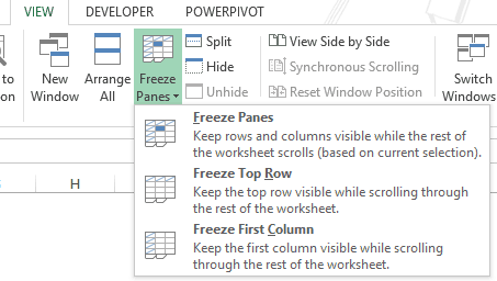
It shows three options in the Freeze Panes drop-down:

• Freeze Panes: It freezes the rows as well as the columns.
• Freeze Top Row: It freezes all the rows above the active cell.
• Freeze First Column: It freezes all the columns to the left of the active cell.

You can use these options to lock rows or columns (or both) into panes in Excel.

Let’s see how to use these options to Freeze Panes in Excel while working with large data sets:

Freezing Row(s) in Excel

If you are working with a dataset that has headers at the top row and a dataset that spans hundreds of rows, as soon as you scroll down, the headers/labels would disappear.

Something as shown below:

In such cases, it’s a good idea to freeze the header row so that these are always visible to the user.

In this section, you’ll learn how to:

• How to Freeze the top row.
• How to Freeze more than one row.
• How to Unfreeze rows.

Freeze the Top Row in Excel

Here are the steps to freeze the first row in your dataset:

• Click the ‘View’ tab.
• In the Zoom category, click on the Freeze panes drop down
  
• Click on the ‘Freeze Top Row’ option.
  • This will freeze the first row of the data set. You would notice that a gray line now appears right below the first row.

Now when you scroll down, the row that has been frozen would always be visible. Something as shown below:

Freeze/Lock More than One Row in Excel

If you have more than one header rows in your dataset, you may want to freeze all of it.

Here is how to freeze rows in Excel:

• Select the left-most cell in the row which is just below the headers row.
• Click the ‘View’ tab.
• In the Zoom category, click on the Freeze panes drop down

• In the Freeze Panes drop-down, select Freeze Panes.
• This will freeze all the rows above the selected cell. You would notice that a gray line now appears right below the rows that have been freezed.

Now when you scroll down, all the header rows would always be visible. Something as shown below:

Also read: How to Freeze Multiple Columns in Excel?

Unfreeze Rows in Excel

To unfreeze row(s):

• Click the ‘View’ tab.
• In the Zoom category, click on the Freeze panes drop down
  
• In the Freeze Panes drop-down, select the option to Unfreeze Panes.

Excel Freeze Panes Options – Freezing Column(s)

If you are working with a dataset that has headers/labels in a column and the data is spread across many columns, as soon as you scroll to the right, the header would disappear.

Something as shown below:

In such cases, it’s a good idea to freeze the left-most column so that the headers are always visible to the user.

In this section, you’ll learn how to:

• How to Freeze the Left-most Column.
• How to Freeze more than one Column.
• How to Unfreeze Columns.

Freeze/Lock the Left-Most Column in Excel

Here is how to freeze the left-most column:

• Click the ‘View’ tab.
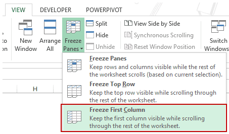
• In the Zoom category, click on the Freeze panes drop down
  
• In the Freeze Panes drop-down, select Freeze First Column.
• This will freeze the left-most column of the data set. You would notice that a gray line now appears at the right border of the left-most column.

Now when you scroll down, the left-most column would always be visible. Something as shown below:

Additional Notes:

• Once you freeze a column, you can not use Control + Z to unfreeze it. You need to use the unfreeze option in the Freeze Panes drop-down.
• If you insert a column to the left of the column that has been frozen, even the inserted column is frozen.

Freeze/Lock More than One Column in Excel

If you have more than one column that contains headers/labels, you may want to freeze all of it.

Here is how to do this:

• Select the top-most cell in the column which is right next to the columns that contain headers.
• Click the ‘View’ tab.
• In the Zoom category, click on the Freeze panes drop-down

• In the Freeze Panes drop-down, select Freeze First Column.
• This will freeze all the columns to the left of the selected cell. You would notice that a gray line appears to the right of the columns that have been frozen.

Now when you scroll to the right, all the columns with headers would always be visible. Something as shown below:

Unfreeze Columns in Excel

To unfreeze column(s):

• Click the ‘View’ tab.
• In the Zoom category, click on the Freeze panes drop-down
  
• In the Freeze Panes drop-down, select the option to Unfreeze Panes.

Freezing Both Row(s) & Column(s)

In most of the cases, you would have the headers/labels in rows as well as in columns. In such cases, it makes sense to freeze both rows and columns.

Here is how you can do this:

• Select a cell just below the rows and right next to the column that you want to freeze.
  • For example, if you want to freeze two rows (1 & 2) and two columns (A & B), select cell C3.
• Click the ‘View’ tab.
• In the Zoom category, click on the Freeze panes drop-down
  
• Select the Freeze Panes option from the drop-down.
• This will freeze the column(s) to the left of the selected cell and row(s) above the selected cell. You would notice two gray lines appear –  one right next to the frozen columns and the other right below the frozen rows.

Now when you scroll down or to the right, the frozen rows and columns would always be visible. Something as shown below:

You can unfreeze the frozen rows and columns at one go. Here are the steps:

• Click the ‘View’ tab.
• In the Zoom category, click on the Freeze panes drop down
  
• In the Freeze Panes drop-down, select the option to Unfreeze Panes.

Notes:

• Apart from working with large data sets, one practical use where you may want to freeze panes in Excel is when you are creating dashboards. You can freeze rows and columns that contain the dashboard so that the user can’t scroll away and the dashboard is always visible.
• A good practice while working with large data sets is to convert it into Excel Tables. By default, all the row headers in Excel Tables are always visible when you scroll within the dataset.

You May Also Like the Following Excel Tutorials:

• Excel Data Entry Tips
• How to Lock Cells in Excel.
• How to Lock Formulas in Excel.
• Compare Columns in Excel
• Move Rows and Columns in Excel
• Delete Blank Rows in Excel
• Highlight Rows Based on a Cell Value in Excel
• How to Turn OFF Scroll Lock in Excel?