Find the Closest Match in Excel (using Formulas)

Excel functions can be extremely powerful if you get a hang of combining different formulas. Things that might have seemed impossible would suddenly start looking like a child’s play.

One such example is to find the closest match of a lookup value in a dataset in Excel.

There are a couple of useful lookup functions in Excel (such as VLOOKUP & INDEX MATCH), which can find the closest match in a few simple cases (as I will show with examples below).

But the best part is that you can combine these lookup functions with other Excel functions to do a lot more (including finding the closest match of a lookup value in an unsorted list).

In this tutorial, I will show you how you find the closest match of a lookup value in Excel with lookup formulas.

Find the Closest Match in Excel

There can be many different scenarios where you need to look for the closest match (or the nearest matching value).

Below are the examples I will cover in this article:

1. Find the commission rate based on sales
2. Find the best candidate (based on the closest experience)
3. Finding the next event date

Let’s get started!

Click here to download the example file

Find Commission Rate (Looking for the Closest Sales Value)

Suppose you have a dataset as shown below where you want to find the commission rates of all the sales personnel.

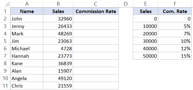
The commission is assigned based on the sale value. And this is calculated using the table on the right.

For example, if a salesperson does the total sales of 5000, then the commission is 0% and if he/she does the total sales of 15000 then the commission is 5%.

To get the commission rate, you need to find the closest sale range just lower than The sale value. For example, for 15000 sale value, the commission would be of 10,000 (which is 5%) and for sale value of 25000, the commission rate would be of  20,000 (which is 7%).

To find the closest sale value and get the commission rate, you can use the approximate match in VLOOKUP.

The below formula would do this:

=VLOOKUP(B2,$E$2:$F$6,2,1)

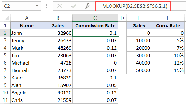
Note that in this formula, the last argument is 1, which tells the formula to use an approximate lookup. This means that the formula would go through the sale values in column E and find the value which is just lower than the lookup value.

Then the VLOOKUP formula will give the commission rate for this value.

Click here to download the example file

Find the best candidate (based on the closest experience)

In the above example, the data needed to be sorted in ascending order. But there could be cases where the data is not sorted.

So let’s cover an example and see how we can find the closest match in Excel using a combination of formulas.

Below is a sample data set where I need to find the employee name that has the work experience closest to the desired value. The desired value in this case in 2.5 years.

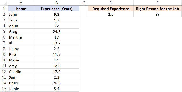
Note that the data is not sorted. Also, the closest experience can be either less or more than the give experience. For example, 2 years and 3 years are both equally close (difference of 0.5 years).

Below is the formula that will give us the result:

=INDEX($A$2:$A$15,MATCH(MIN(ABS(D2-B2:B15)),ABS(D2-$B$2:$B$15),0))

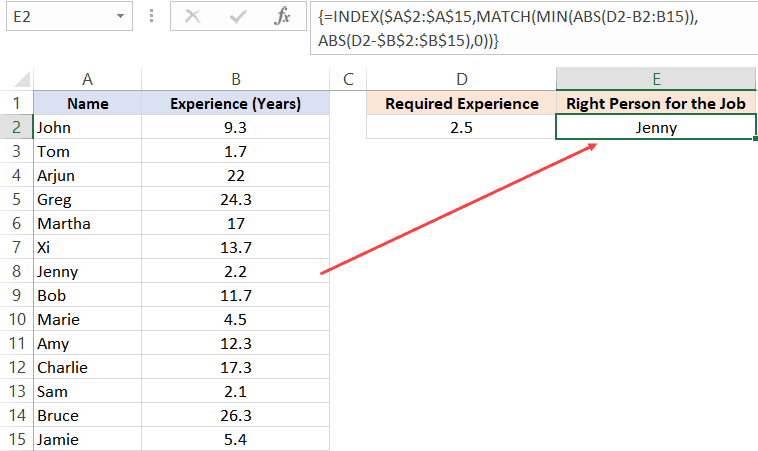
The trick in this formula is to change the lookup array and the lookup value to find the minimum experience difference in required and actual values.

Let’s first understand how you would do it manually (and then I will explain how this formula works).

When doing this manually, you will go through each cell in column B and find the difference in the experience between what is required and the one that a person has. Once you have all the differences, you will find the one which is minimum and fetch the name of that person.

This is exactly what we are doing with this formula.

Let me explain.

The lookup value in the MATCH formula is MIN(ABS(D2-B2:B15)).

This part gives you the minimum difference between the given experience (which is 2.5 years) and all the other experiences. In this example, it returns 0.3

Note that I have used ABS to make sure I am looking for the closest (which can be more or less than the given experience).

Now, this minimum value becomes our lookup value.

The lookup array in the MATCH function is ABS(D2-$B$2:$B$15).

This gives us an array of numbers from which 2.5 (the required experience) has been subtracted.

So now we have a lookup value (0.3) and a lookup array ({6.8;0.8;19.5;21.8;14.5;11.2;0.3;9.2;2;9.8;14.8;0.4;23.8;2.9})

MATCH function finds the position of 0.3 in this array, which is also the position of the person’s name who has the closest experience.

This position number is then used by the INDEX function to return the name of the person.

Note: In case there are multiple candidates that have the same minimum experience, the above formula is going to give the name of the first matching employee.

Find the Next Event Date

This is another example where you can use lookup formulas to find the next date of an event based on the current date.

Below is the dataset where I have event names and the event dates.

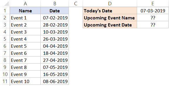
What I want is the name of the next event and the event date for this upcoming event.

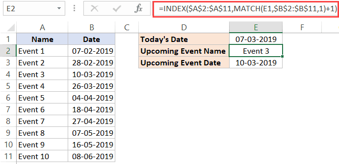
Below is the formula that will give the upcoming event name:

=INDEX($A$2:$A$11,MATCH(E1,$B$2:$B$11,1)+1)

And below formula will give the upcoming event date:

=INDEX($B$2:$B$11,MATCH(E1,$B$2:$B$11,1)+1)

Let me explain how this formula works.

To get the event date, the MATCH function looks for the current date in column B. In this case, we are not looking for an exact match, but an approximate one. And hence, the last argument of the MATCH function is 1 (which finds the largest value that is less than or equal to the lookup value).

So the MATCH function would return the position of the cell which has the date which is just less than or equal to the current date. So the next event, in this case, would be in the next cell (as the list is sorted in ascending order).

So to get the upcoming event date, just add one to the cell position returned by the MATCH function, and it will give you the cell position of next event date.

This value is then given by the INDEX function.

To get the event name, the same formula is used, and the range in INDEX function is changed from column B to column A.

Click here to download the example file

These are three examples that show how to find the closest matching value in Excel using lookup formulas.

You May Also Like the Following Excel Tips/Tutorials

• Get the Last Number from a List using VLOOKUP Function.
• Get Multiple Lookup Values Without Repetition in a Single Cell.
• VLOOKUP Vs. INDEX/MATCH
• Excel INDEX MATCH
• Find the Last Occurrence of a Lookup Value a List in Excel
• Find and Remove Duplicates in Excel
• Conditional Formatting.