
If you have data split across two columns, like first names in one and last names in another, you may want to pull them together into a single column.
And the tricky part is usually getting the spacing right so the names don’t end up squished together.
But nothing to worry about. It’s a quick job once you know which approach to use.
In this article, I’ll show you a few easy ways to combine two columns in Excel, with a space or a comma in between.
Combine Two Columns Using the Ampersand (&) Operator
The simplest way to join two columns is the ampersand operator (&). You just glue the two cells together and tell Excel what to put in between them.
This is the method I reach for most of the time because it’s short and it works in every version of Excel.
Let me show you how it works.
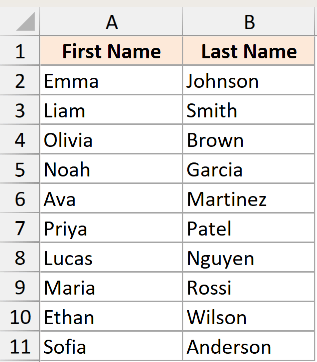
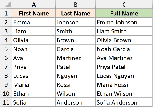
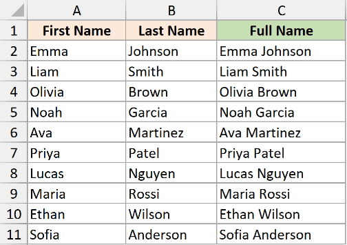
Below I have a dataset with first names in column A and last names in column B. I want the full name in column C.

To combine the two with a space in between, here is the formula:
=A2:A11&" "&B2:B11
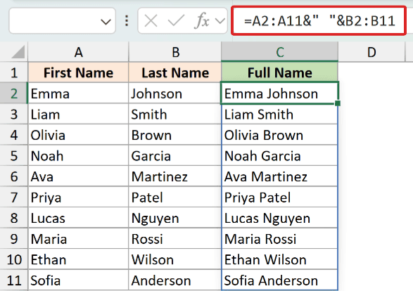
This spills the full names down column C in one go, with Emma Johnson in C2 and the rest filling in below it.
How does this formula work?
The & operator joins whatever is on either side of it into one piece of text.
So A2:A11&B2:B11 would give you EmmaJohnson with no gap.
To add the space, I’ve slipped " " (a space inside double quotes) between the two ranges. Because I’ve referenced the whole ranges A2:A11 and B2:B11 instead of single cells, the formula spills down the entire column on its own in Excel 365 and Excel 2021.
You can put any text you like inside those quotes. If you want a comma and a space instead of just a space, use this formula:
=A2:A11&", "&B2:B11
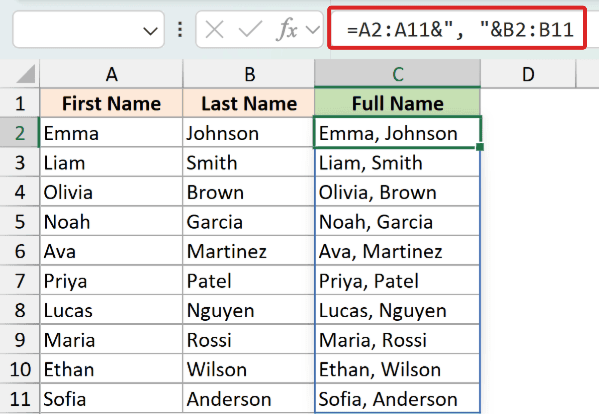
This spills Emma, Johnson and the rest down the column. A comma reads nicely when you’re joining something like a city and a state, for example New York, NY.
Because it’s a dynamic array, you enter the formula once in C2 and it fills the whole column for you. On older versions of Excel without dynamic arrays, use the single-cell form =A2&" "&B2 and copy it down the column instead.
Using TEXTJOIN to Combine First and Last Name
TEXTJOIN does the same job, but it lets you set the separator once and then list the cells you want to combine. It also has a handy option to skip blank cells.
This one is great when you’re joining more than two columns, or when some cells might be empty.
Same data as before. First names are in column A, last names in column B, and I want the full name in column C.
Here is the formula to combine the names with a space:
=TEXTJOIN(" ",TRUE,A2,B2)
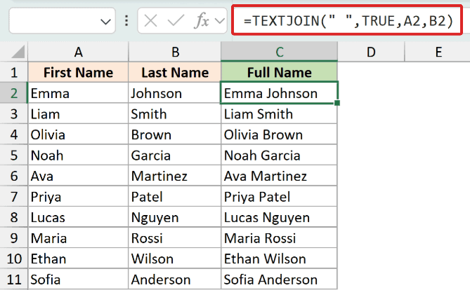
This returns Emma Johnson in cell C2.
How does this formula work?
TEXTJOIN takes three things in this example:
- The first argument is the delimiter. I’ve used
" "so a space goes between each value. - The second argument is ignore_empty. I’ve set it to
TRUE, so if a cell is blank, Excel skips it instead of leaving a stray extra space. - After that, you list the cells you want to join (here, A2 and B2).
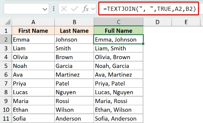
To use a comma instead, just change the delimiter:
=TEXTJOIN(", ",TRUE,A2,B2)
The reason TEXTJOIN really shines is that ignore_empty setting. If you’re joining several columns and a middle name is missing for some people, TEXTJOIN won’t leave double spaces where the blank was.
Pro Tip: TEXTJOIN is available in Excel 2019 and Microsoft 365. If you’re on an older version, use the ampersand method instead.
Merge Columns Using the CONCAT Function
CONCAT is another function that joins text together. It’s the newer replacement for the old CONCATENATE function.
Unlike TEXTJOIN, CONCAT doesn’t have a built-in separator argument. So if you want a space or comma, you add it yourself the same way you do with the ampersand.
I’m using the same dataset here too, with the first name in column A and the last name in column B. The goal is the same, a full name in column C.
Here is the formula:
=CONCAT(A2," ",B2)
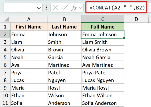
This returns Emma Johnson. For a comma, swap the " " for ", " in the middle.
How does this formula work?
CONCAT joins everything you list inside the brackets, in order. So I’ve placed " " between A2 and B2 to drop a space between the first and last name.
CONCAT replaced CONCATENATE in Excel 2019. CONCATENATE still works for backward compatibility, so older files won’t break, but Microsoft recommends using CONCAT (or TEXTJOIN) going forward.
Using Flash Fill
Flash Fill is a nice option if you’d rather not deal with formulas at all. You type the result you want once, and Excel figures out the pattern and fills the rest for you.
Keep in mind that Flash Fill gives you plain text, not a formula. So if you change a name in column A later, the combined column won’t update on its own.
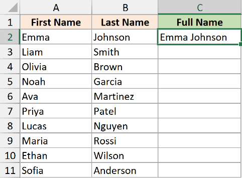
Here’s the starting point again. Column A has the first names, column B has the last names, and column C is where I want the combined name.
Here are the steps to combine two columns using Flash Fill:
- In the first cell of the column where you want the result (C2), type the combined value yourself, for example Emma Johnson.
- Select cell C3 (the cell right below what you just typed).
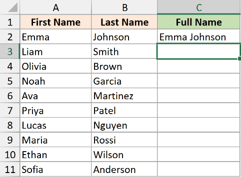
- Press Ctrl + E on your keyboard.
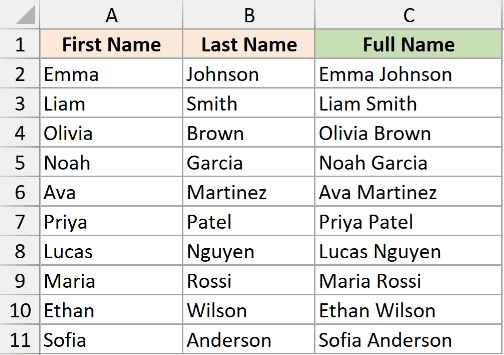
Excel reads the example you typed, picks up the pattern, and fills in the full names for the rest of the rows.
If you’d rather not use the shortcut, you can do the same thing from the ribbon. Go to the Data tab and click Flash Fill in the Data Tools group.
Pro Tip: If Flash Fill doesn’t fill the column, type the second example in C3 too, then select C4 and press Ctrl + E again. Two examples usually give Excel enough to lock onto the pattern.
Merge Columns Using Power Query
Power Query is the one method here that stays connected to your source data. It doesn’t update on its own, but once it’s set up, you can refresh the result in a click whenever your data changes.
That makes it a good fit for data you update regularly, or for large datasets where you’d rather not put a formula in every row.
Power Query is built into Excel 2016 and later on Windows, and in Microsoft 365 on both Windows and Mac.
The source data is the same two columns: first names in column A and last names in column B.
We can load this data into the Power Query editor and do the transformation there. Once done we can load that table back into Excel.
Power Query works on an Excel Table, so the first step is to turn the data into one.
Here is how to combine two columns with Power Query:
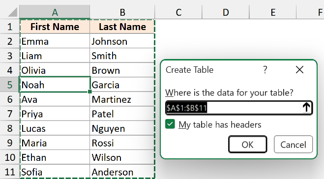
- Convert your data into an Excel Table. Select any cell in the data and press Ctrl + T. In the Create Table dialog, make sure My table has headers is ticked, then click OK.
- With the table selected, go to the Data tab and click From Table/Range. Excel opens the two columns in the Power Query Editor.
- Click the header of the first column (First Name), then hold Ctrl and click the second column (Last Name) so both are selected. The order you click them is the order they get joined.
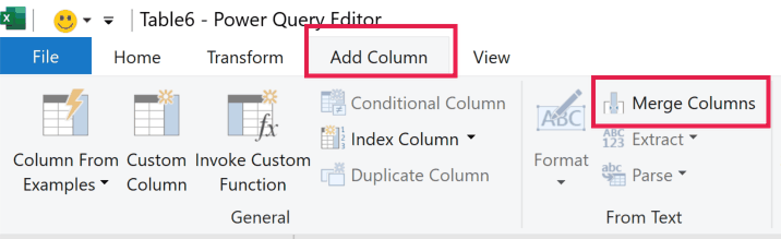
- Go to the Add Column tab and click Merge Columns. This keeps your First Name and Last Name columns and adds the combined one next to them.
- In the Merge Columns dialog, pick a Custom Separator and enter comma followed by space in the field below, and then type a name like Full Name for the new column, and click OK.
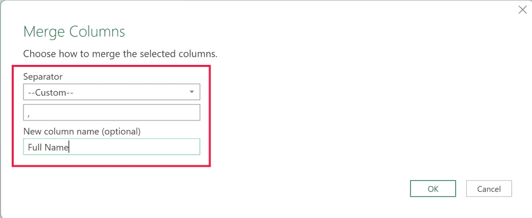
This will combine the two columns and you will see a new column appear with the full names

- On the Home tab, click Close & Load. Power Query loads a new table on a new sheet with your First Name, Last Name, and combined Full Name columns.
When your source data changes, refresh the query: right-click the loaded table and choose Refresh (or go to Data > Refresh All). The combined column updates to match, and any new rows come along too.
The formula methods update automatically when you edit a name, but they don’t reach new rows on their own.
Flash Fill, Notepad, and the macro don’t update at all. Power Query covers both with a refresh.
Pro Tip: If you only want the single combined column and don’t need the originals, use Merge Columns on the Transform tab instead. It turns the two selected columns into one.
Using Notepad to Combine Columns
Here’s a quick trick that skips both formulas and Power Query.
You copy the two columns into Notepad, swap the tab between them for a space or comma, and paste the result back. It’s handy for a fast one-time combine.
Like the other methods, I have the first names in column A and the last names in column B, and I want them combined in column C.
- Select both columns of data (here A2:B11) and press Ctrl + C to copy.

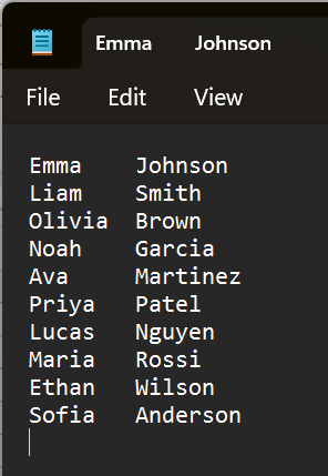
- Open Notepad and press Ctrl + V to paste. Excel drops a tab between the two columns.
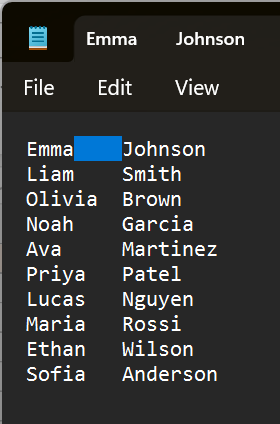
- Highlight the gap (the tab) between any first and last name and copy it with Ctrl + C.
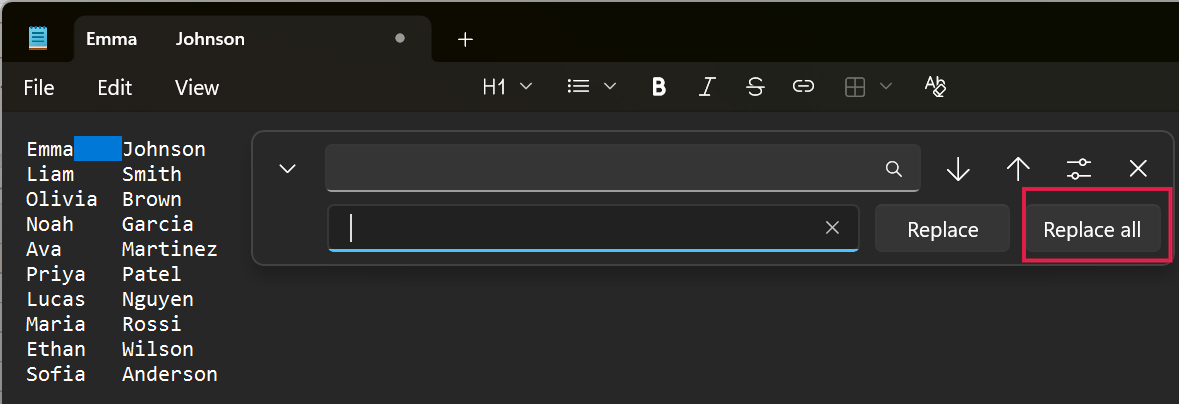
- Then press Ctrl + H to open Replace, click in the Find what box and paste the tab with Ctrl + V, type a space (or a comma) in Replace with, and click Replace All.
- Press Ctrl + A to select all the text, copy it, and paste it back into the empty column in Excel.
Like Flash Fill, this gives you plain text, not a formula, so it won’t update if the original names change later.
Using a VBA Macro
If you combine columns often, a short macro can do the whole job in one click.
This is the most advanced option here, so it’s really for automating a repeat task rather than a one-off. Like Flash Fill, it writes plain values, not formulas.
Same setup once more. The first names are in column A, the last names in column B, and column C is where the full name should go.
Here are the steps to combine two columns with a macro:
- Press Alt + F11 to open the Visual Basic Editor.
- In the editor, click Insert in the menu and choose Module.
- Copy the code below and paste it into the module window.
Sub CombineColumns()
    Dim i As Long
    Dim lastRow As Long
    lastRow = Cells(Rows.Count, 1).End(xlUp).Row
    For i = 2 To lastRow
        Cells(i, 3).Value = Cells(i, 1).Value & " " & Cells(i, 2).Value
    Next i
End Sub- Press F5 (or click the green Run button), then close the editor and go back to your sheet. Column C now has the combined names.
How does this macro work?
lastRowfinds the last filled row in column A, so the macro knows where to stop.- The loop runs from row 2 down to that last row.
- For each row, it joins column A (
Cells(i, 1)) and column B (Cells(i, 2)) with a space and drops the result into column C (Cells(i, 3)).
To use a comma instead of a space, change " " to ", ". And to keep the macro for next time, save the file as a macro-enabled workbook (.xlsm).
Why Merge & Center Doesn’t Combine Columns (It Deletes Your Data)
If you’ve ever tried Excel’s Merge & Center button (on the Home tab) to join two columns, you’ve probably seen it go wrong.
Merge & Center is built for formatting, like centering a title across several cells. It isn’t built for combining data.
When you select two cells that both have values and click Merge & Center, Excel keeps only the upper-left value and discards the rest. You’ll even get a warning telling you so.
So for joining something like first and last names, skip Merge & Center and use one of the methods above instead.
Things to Keep in Mind
- The result is always text. Even if you combine two columns of numbers, the joined value becomes text, so don’t expect to add it up or run number formats on it.
- To delete the original columns, convert the formulas first. The combined column depends on columns A and B, so deleting them breaks the result. Copy the combined column, then right-click and use Paste Special > Values to turn the formulas into plain text before you delete the originals.
- Watch out for double spaces. If a cell is empty and you’re using the ampersand or CONCAT, you can end up with an extra space. TEXTJOIN with ignore_empty set to TRUE avoids this for you.
- Only the ampersand formula spills the whole column on its own. TEXTJOIN and CONCAT work one row at a time, so you enter them in the first cell and copy them down. Flash Fill, Power Query, Notepad, and the macro fill the column for you.
In this article, I showed you several easy ways to combine two columns in Excel using a space or a comma, from the simple ampersand operator to TEXTJOIN, CONCAT, Flash Fill, Power Query, Notepad, and a VBA macro.
I hope you found this article helpful.
Other Excel Articles You May Also Like:


