

If you want a formula that points to a cell or range that shifts based on a value you feed it, OFFSET is the function you want.
It returns a reference a set number of rows and columns away from a starting cell, and you can size that reference into a full range.
One heads-up: OFFSET is a volatile function. It recalculates on every change in the workbook, and it is not a dynamic array function you would reach for to spill results.
It returns a reference, which you usually feed into another function like SUM or AVERAGE.
In this article, I’ll show you how to use the OFFSET function with several practical examples.
OFFSET Function Syntax
Here is the syntax of the OFFSET function:
=OFFSET(reference, rows, cols, [height], [width])
- reference – The starting cell or range that OFFSET counts from. This is your anchor point.
- rows – How many rows to move from the reference. A positive number goes down, a negative number goes up.
- cols – How many columns to move from the reference. A positive number goes right, a negative number goes left.
- height – Optional. How many rows tall the returned range should be. If you leave it out, it matches the reference.
- width – Optional. How many columns wide the returned range should be. If you leave it out, it matches the reference.
How the OFFSET Function Works (a Chess Analogy)
OFFSET trips up a lot of people at first, so here is a mental model that makes it click.
Think of the rook in chess. From wherever it sits, it moves in straight lines: so many squares up or down, so many squares left or right, but never diagonally.

Say the rook sits on square D5 and you want to move it to F7. You would tell it to go two squares down and two squares to the right.
OFFSET works the exact same way. Give it a starting cell, tell it how many rows to move down and how many columns to move right, and it lands on a new cell.
The formula =OFFSET(D5, 2, 2) starts at D5, moves 2 rows down and 2 columns right, and returns whatever sits in F7.
Once you picture that rook moving around the board, the rows and cols arguments stop feeling abstract.
When to Use the OFFSET Function
Use OFFSET when you need to:
- Pull a value that sits a certain distance from a known starting cell.
- Build a range that grows or shrinks on its own as you add or remove data.
- Sum, average, or count a window of cells that moves based on an input.
- Create a dynamic named range for a drop-down list or a chart.
Let me show you a few practical examples of how this works.
Example 1: Grab a Value a Set Distance Away
Let’s start with a simple example.
Below is a dataset with website stats. Column A has the month, column B has the number of visitors, and column C has the number of signups for six months.
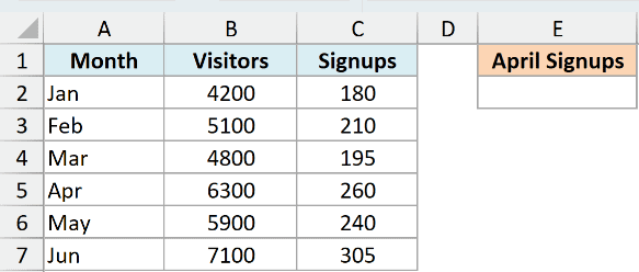
I want to pull the signups for April, starting from the top-left corner of the table in cell A1.
Here is the formula:
=OFFSET(A1, 4, 2)
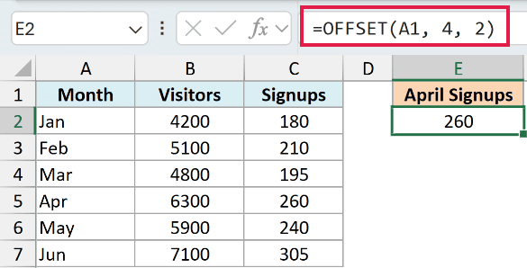
Here, OFFSET starts at cell A1, moves down 4 rows to the April row, and then moves 2 columns to the right into the Signups column.
That lands on cell C5, so the formula returns 260. Change either number and the formula points somewhere else.
Example 2: Return a Whole Range by Setting Height and Width
Now let’s see how the last two arguments turn OFFSET into a range instead of a single cell.
Below is a small grid of quarterly sales by product. Column A has the product, and columns B to E hold the Q1 to Q4 sales for four products.
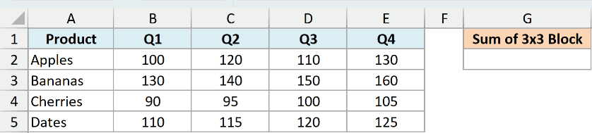
I want the total of the first three products across Q1, Q2, and Q3, which is the 3-by-3 block starting at B2.
Here is the formula:
=SUM(OFFSET(A1, 1, 1, 3, 3))
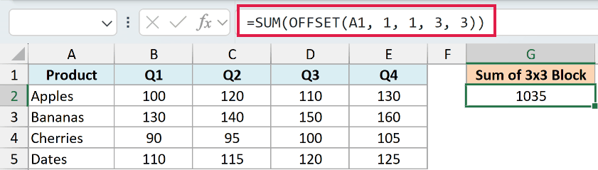
How this formula works, one argument at a time:
- reference is A1, the anchor in the top-left corner.
- rows is 1, so OFFSET moves down 1 row to row 2.
- cols is 1, so it moves right 1 column to column B, landing the start at B2.
- height is 3, which makes the reference 3 rows tall.
- width is 3, which makes it 3 columns wide, so the reference becomes the block B2:D4.
- SUM then adds those 9 values, giving 1035.
Pro Tip: To see exactly which cells OFFSET grabs, click into the formula, select just the OFFSET(…) part, and press F9. Excel shows the array of values it points to. Press Esc to undo before you leave the cell. In Excel 365, typing =OFFSET(A1, 1, 1, 3, 3) on its own spills the whole block, while older versions return a #VALUE! error because one cell cannot show a range.
Example 3: Sum the Last N Values with OFFSET
Here’s a scenario I run into a lot with reports that keep growing.
Below is a list of weekly revenue. Column A has the week and column B has the revenue, and a new row gets added at the bottom every week.
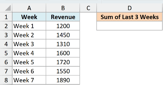
I want to always sum the last 3 weeks of revenue, even as new weeks are added below.
Here is the formula:
=SUM(OFFSET(B1, COUNTA(B:B)-3, 0, 3, 1))
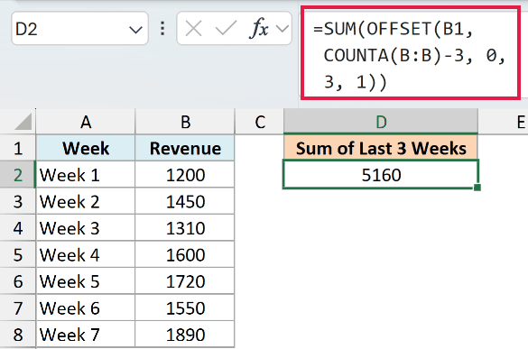
How this formula works:
- COUNTA(B:B) counts the filled cells in column B, which is 8 here (the header plus 7 weeks).
- Subtracting 3 gives 5, so OFFSET moves down 5 rows from B1 and lands on B6, the third week from the bottom.
- The height of 3 and width of 1 make OFFSET return the range B6:B8.
- SUM then adds that range, giving 5160.
When a new week is added, COUNTA goes up by one and the window slides down to the newest three weeks on its own.
Pro Tip: COUNTA assumes there are no blank cells in the column. If your data has gaps, the count will be off and the window will land on the wrong rows.
Example 4: Build a Dynamic Named Range with OFFSET
Now let’s look at something a bit more useful.
Below is a list of products in column A that you keep adding to over time. You want a drop-down list (or a chart) that always includes every product, without editing the source range each time.
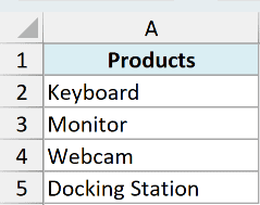
I want a named range that automatically expands to cover every product as the list grows.
In the Name Manager, create a name (say, ProductList) that refers to this formula:
=OFFSET($A$2, 0, 0, COUNTA($A:$A)-1, 1)
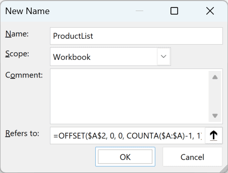
Here, OFFSET starts at the first product in A2 and stays put with 0 rows and 0 columns of movement. The height is set by COUNTA($A:$A)-1, which counts the filled cells in column A and subtracts 1 for the header.
With four products, that height is 4, so the name points to A2:A5. Add a fifth product and it stretches to A2:A6 on its own.
Pro Tip: For a dynamic range that isn’t volatile, an INDEX-based version like =$A$2:INDEX($A:$A, COUNTA($A:$A)) usually does the same job without recalculating on every change. It’s the better default in big workbooks.
Example 5: Sum a Variable Window of Rows
Let’s step it up with a window you control from input cells.
Below is a table of monthly sales for the year. Column A has the month and column B has the sales. Off to the side, cell E2 holds a start month number and cell E3 holds how many months to add up.
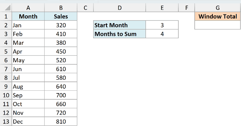
I want to sum a block of months that starts wherever E2 says and runs for as many months as E3 says.
Here is the formula:
=SUM(OFFSET(B1, E2, 0, E3, 1))
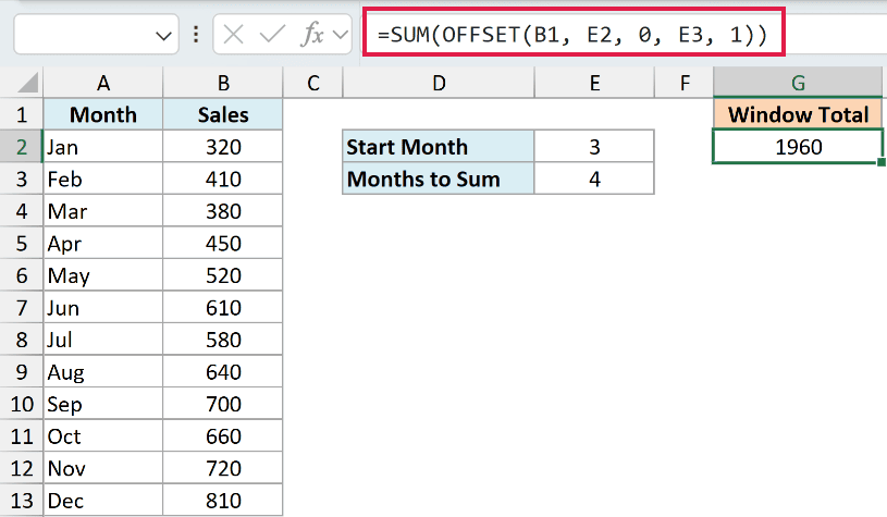
How this formula works:
- The rows argument is E2 (3 here), so OFFSET moves down 3 rows from B1 and lands on B4, the March sales.
- The height argument is E3 (4 here), so the returned range is 4 rows tall: B4:B7.
- SUM adds March through June, giving 1960.
Change E2 to slide the window to a different starting month, or change E3 to make it cover more or fewer months. The total updates instantly.
Example 6: Get the Last Value in a Column
This next one is handy for a running log where you always want the newest entry.
Below is an account balance log. Column A has the date and column B has the balance after each transaction, with the latest balance at the bottom.
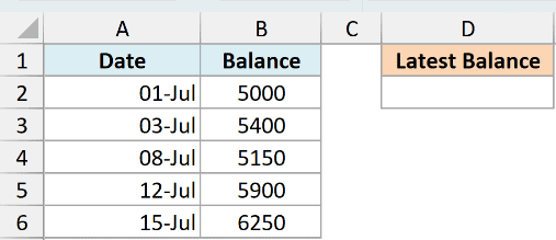
I want to pull the most recent balance, wherever the bottom of the list happens to be.
Here is the formula:
=OFFSET(B1, COUNTA(B:B)-1, 0)
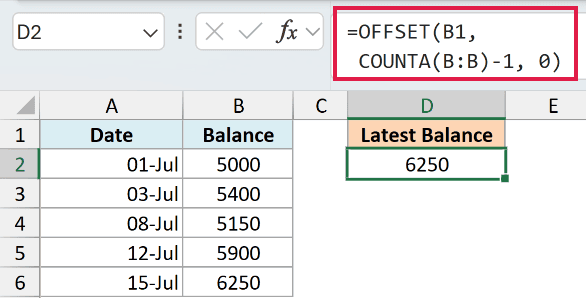
In the above formula, COUNTA(B:B) counts the filled cells in column B, which is 6 (the header plus 5 balances).
Subtracting 1 gives 5, so OFFSET moves down 5 rows from B1 to the last filled cell, B6, and returns 6250. As you add more rows, it keeps grabbing the newest balance.
Pro Tip: In Excel 365 you can get the last value with the newer TAKE function, like =TAKE(B2:B6, -1), which isn’t volatile. OFFSET stays useful when you need this to work in older versions of Excel.
Example 7: Average a Moving 2D Block
Let’s finish with a reference that moves in two directions at once.
Below is a small grid of monthly sales by region. Column A has the month, and columns B, C, and D hold the sales for North, South, and East.
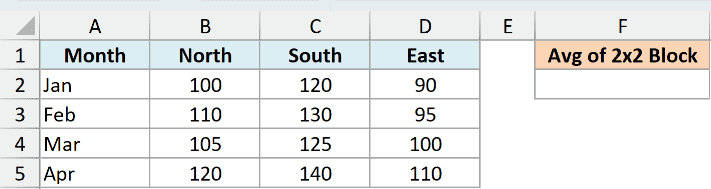
I want the average of a 2-by-2 block covering the first two months for North and South.
Here is the formula:
=AVERAGE(OFFSET(A1, 1, 1, 2, 2))
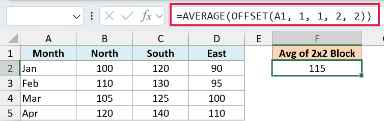
Here, OFFSET starts at A1, moves down 1 row and right 1 column to land on B2. The height of 2 and width of 2 then stretch the reference into the block B2:C3.
That block holds 100, 120, 110, and 130, so AVERAGE returns 115. Adjusting the row, column, height, or width slides or resizes the block.
Tips & Common Mistakes
- OFFSET is volatile. It recalculates every time anything in the workbook changes, not just when its own inputs change. A handful is fine, but hundreds of OFFSET formulas can slow a large workbook to a crawl.
- Watch for the #REF! error. If the rows or cols argument pushes the reference off the edge of the worksheet, OFFSET returns #REF!. Keep your offsets inside the data.
- Mind the sign. Positive rows go down and positive cols go right. Negative values move up and left, which is easy to forget.
- COUNTA and blank cells don’t mix. The dynamic-range trick relies on a column with no gaps. A blank cell in the middle throws the count off and the range lands in the wrong place.
- Consider INDEX or a Table instead. INDEX can build the same dynamic ranges without being volatile, and an Excel Table with structured references often removes the need for OFFSET entirely. In Excel 365, FILTER and TAKE cover many of these jobs too.
OFFSET is one of those functions that looks odd at first but clicks once you see it as a moving pointer.
You give it a starting cell, tell it how far to move, and optionally how big a range to grab. It hands back a reference you can drop into SUM, AVERAGE, or a named range.
Just keep the volatility in mind, and reach for INDEX or the newer dynamic array functions when they’ll do the job with less overhead.
Other Excel Articles You May Also Like:
