

If you want to find the smallest number in a list of values, whether it’s the lowest price, the earliest date, or the smallest quantity, the MIN function is the quickest way to do it.
MIN returns a single value, but it also works well inside dynamic array formulas like =MIN(FILTER(...)), so you can pull the lowest value from a filtered set too.
Follow along with the example file
MIN Function Examples.xlsx
MIN Syntax
Here is the syntax of the MIN function:
=MIN(number1, [number2], ...)
- number1 – The first number, cell, or range you want to find the minimum from. This is required.
- number2, … – Additional numbers, cells, or ranges. These are optional. You can pass up to 255 arguments.
MIN scans everything you give it and returns the smallest number. It ignores empty cells, text, and logical values (TRUE/FALSE) inside a range, so a stray label in your data won’t break the formula. Errors in the referenced range are not ignored.
When to Use MIN in Excel
Use the MIN function when you need to:
- Find the lowest value in a list, such as the cheapest quote or the smallest order.
- Pull the smallest number from several ranges at once.
- Set a ceiling on a value, so it never goes above a limit you decide.
- Find the earliest date in a schedule (dates are just numbers to Excel).
Let me show you a few practical examples of how to use MIN in different situations.
Example 1: Find the Lowest Value in a List
Let’s start with a simple example.
Below is a dataset with eight vendors in column A and the quote each one gave for the same job in column B.
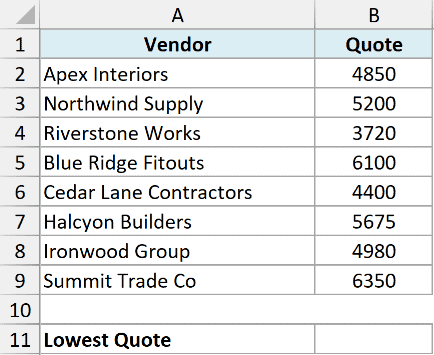
I want to find the lowest quote so I know which vendor is cheapest.
Here is the formula:
=MIN(B2:B9)
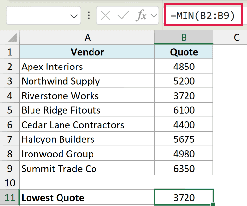
This returns 3720, which is the smallest number in the range B2:B9.
MIN reads every value in the range and hands back the smallest one. That’s the whole job of the function in its most basic form.
3720 tells you the lowest price, but it doesn’t tell you who quoted it. To get the vendor’s name, pair MIN with XLOOKUP.
Here is the formula:
=XLOOKUP(MIN(B2:B9),B2:B9,A2:A9)
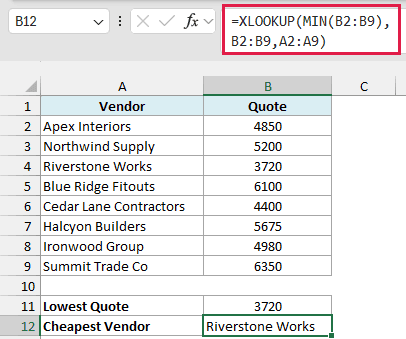
This returns Riverstone Works. MIN(B2:B9) finds 3720, then XLOOKUP looks for it in B2:B9 and returns the vendor name from the same row in A2:A9.
Pro Tip: Excel 2019 and earlier don’t have XLOOKUP. Use =INDEX(A2:A9,MATCH(MIN(B2:B9),B2:B9,0)) to return the same vendor. If two vendors share the lowest quote, both formulas return the first one in the list.
Example 2: Find the Minimum Across Non-Contiguous Ranges
Here’s a scenario where the values you care about aren’t sitting next to each other.
Below is a dataset with five products in column A and their stock counts for each quarter in columns B to E.
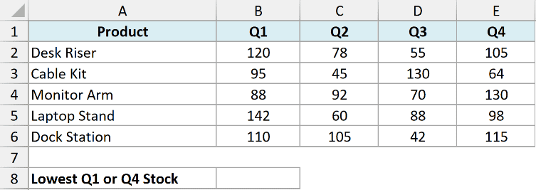
I only want to compare the first quarter (column B) and the last quarter (column E), so I need MIN to look at two separate ranges and skip the columns in between.
Here is the formula:
=MIN(B2:B6, E2:E6)
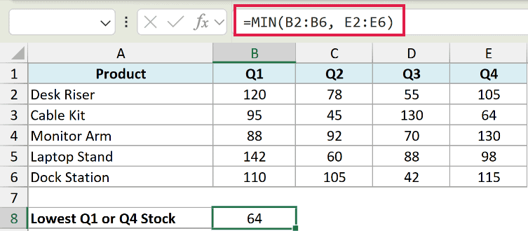
This returns 64, the smallest value found across both ranges.
You can pass MIN as many ranges as you like, separated by commas, and it treats them as one big pool of numbers. The columns in between (C and D) are simply left out.
Example 3: Find the Minimum Based on a Condition
Now let’s find the smallest value that meets a specific condition.
Below is a dataset with airlines in column A, routes in column B, and ticket prices in column C.
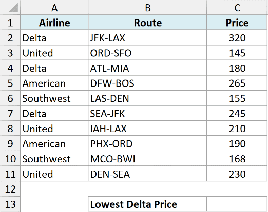
I want the cheapest Delta ticket, so I need the minimum price but only for rows where the airline is Delta.
For this, I’ll use the MINIFS function, which finds the minimum based on one or more conditions.
Here is the formula:
=MINIFS(C2:C11, A2:A11, "Delta")
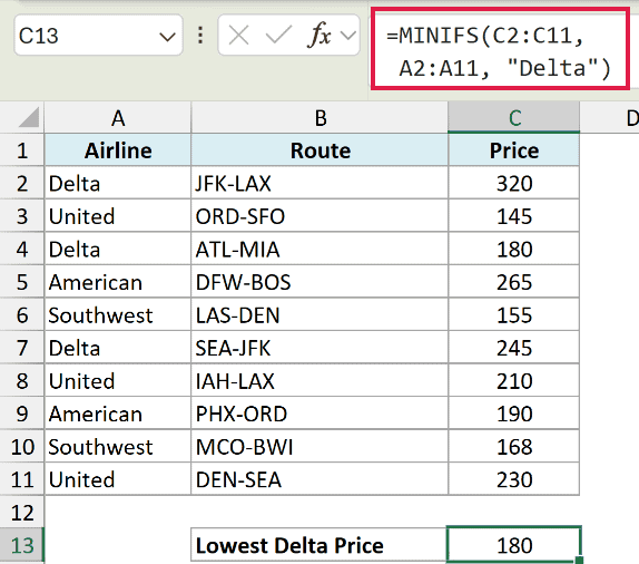
This returns 180, the lowest price among the Delta rows only.
Here is how this formula works:
- C2:C11 is the min_range, the column MINIFS pulls the smallest value from.
- A2:A11 is the range MINIFS checks against the condition.
- “Delta” is the condition. Only rows where column A equals Delta are considered.
Pro Tip: MINIFS is available in Excel 2019 and later, Microsoft 365, and Excel for the web. If you’re on an older version, use an array formula like =MIN(IF(A2:A11="Delta",C2:C11)) entered with Ctrl + Shift + Enter.
Example 4: Find the Minimum Ignoring Zeros (Smallest Positive Value)
MIN ignores blank cells, but it does not ignore zeros. A zero is a real number, so if your data has any, MIN will happily return 0.
Below is a dataset with days of the week in column A and daily sales in column B. On two days the store was closed, so the sales are 0.
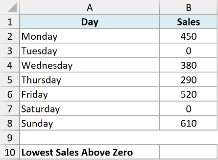
I want the lowest actual sales figure, so I need to skip the zero days and find the smallest value above zero.
Here is the formula:
=MINIFS(B2:B8, B2:B8, ">0")
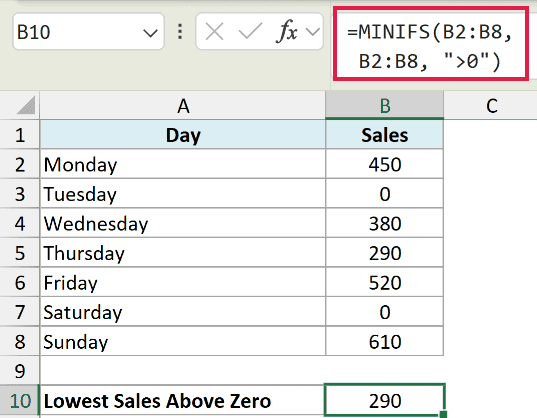
This returns 290. A plain =MIN(B2:B8) would have returned 0 instead.
Here, MINIFS uses the sales column as both the min_range and the criteria range, and the condition “>0” tells it to only consider values greater than zero.
Pro Tip: On versions without MINIFS, use the array formula =MIN(IF(B2:B8>0,B2:B8)) and confirm it with Ctrl + Shift + Enter.
Example 5: Cap a Value at a Maximum Limit
MIN isn’t only for ranges. A common trick is to use it as a ceiling, so a number never rises above a limit you set.
Below is a dataset with employees in column A and the expense amount each one claimed in column B. The company reimburses claims but caps each one at $500.
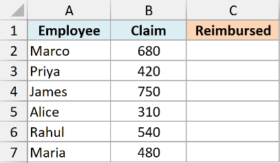
I want the reimbursed amount in column C. If a claim is under $500 it’s paid in full, but anything above $500 is capped at $500.
Here is the formula:
=MIN(500, B2)
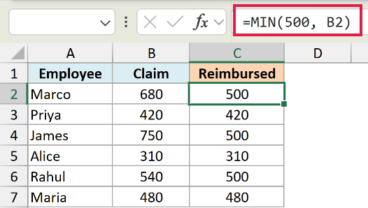
For Marco’s claim of 680, this returns 500, the smaller of the two numbers.
MIN compares the cap (500) with the claim and returns whichever is smaller. When the claim is below 500 you get the claim itself, and when it’s above, you get the cap.
I’ve kept this as a per-row formula so each employee’s claim is capped on its own row.
Example 6: Find the Lowest Value in a Category with FILTER
This is where MIN shows off inside a dynamic array formula.
Below is a dataset with product categories in column A, product names in column B, and revenue in column C.
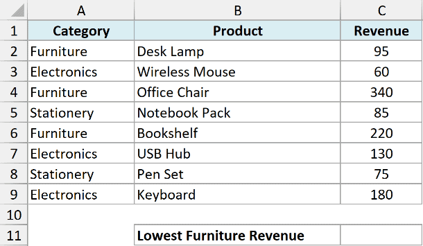
I want the lowest revenue among Furniture products only, and I’ll do it by wrapping the FILTER function inside MIN.
Here is the formula:
=MIN(FILTER(C2:C9, A2:A9="Furniture"))
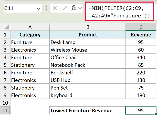
This returns 95, the smallest Furniture revenue in the list.
FILTER first pulls out only the rows where the category is Furniture, and MIN then finds the smallest number in that filtered set. If no row matches, FILTER returns #CALC! because this formula does not supply an empty-result fallback.
Pro Tip: MINIFS from Example 3 does the same job more simply for basic conditions. MINIFS returns 0 when no row matches. Reach for MIN with FILTER when your condition is more complex than MINIFS can handle on its own.
Example 7: Find the Earliest Date
Since Excel stores dates as serial numbers, MIN works on dates just like it does on any other number, and the smallest number is the earliest date.
Below is a dataset with project tasks in column A and their start dates in column B.
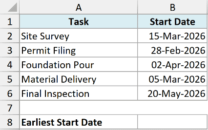
I want to know which task starts first, so I need the earliest start date in the list.
Here is the formula:
=MIN(B2:B6)
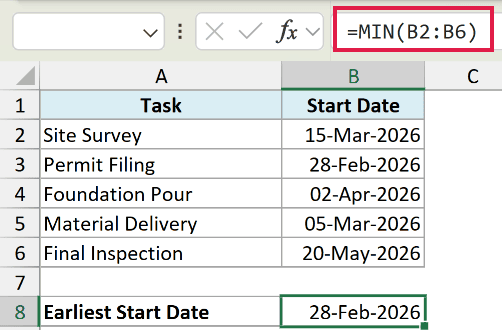
This returns 28-Feb-2026, the earliest date in the range.
The result comes back formatted as a date because the cell is already formatted that way. If you ever see a plain number like 46081 instead, just format the cell as a date and it’ll display correctly.
Tips & Common Mistakes
- MIN ignores text and blanks, but not zeros. Empty cells and text labels inside a range are skipped, but a 0 counts as a real number. Use MINIFS with a “>0” condition when you want the smallest positive value.
- Use MINIFS for conditions. When you need the minimum only for rows that meet a condition, MINIFS is cleaner than a nested MIN and IF. It takes a min_range followed by range and criteria pairs.
- Typed-in logical values are counted. MIN ignores TRUE/FALSE inside a range, but if you type them directly as arguments (like
=MIN(TRUE, 5)), Excel treats TRUE as 1. This rarely matters in practice, but it’s worth knowing. - MIN returns 0 on an empty selection. If none of the arguments contain a number, MIN gives you 0 rather than an error, which can be misleading if you expected a value.
- Need the Nth smallest, not the very smallest? MIN only gives you the single lowest value. For the second or third smallest (or largest), use the SMALL or LARGE function instead.
The MIN function is one of those small tools you’ll reach for constantly once it clicks. You’ve seen how to pull the lowest value from a list, work across separate ranges, add conditions with MINIFS, ignore zeros, cap values, and even find the earliest date.
Combine it with functions like FILTER and it becomes even more flexible for real-world data. Pair it with MAX and you can even calculate the range of your data in a single step.
Other Excel Articles You May Also Like:
