
Excel’s SEQUENCE function is one of those features that might seem simple at first glance, but when you start combining it with other functions, that’s when the real magic happens.
SEQUENCE function does one straightforward thing on its own: it gives you a sequence of numbers.
But trust me, once you see what it can do when paired with other Excel functions, you’ll wonder how you ever managed without it.
In this article, I’m going to walk you through everything you need to know about the SEQUENCE function, including some awesome examples.
Click here to download the example file
Understanding the SEQUENCE Function Syntax
The SEQUENCE function takes four arguments, but you don’t need to use all of them.
Let’s break down each parameter:
=SEQUENCE(rows, [columns], [start], [step])
- Rows (Required): The number of rows to fill
- Columns (Optional): The number of columns to fill
- Start (Optional): The starting value (if omitted, defaults to 1)
- Step (Optional): The increment between values (if omitted, defaults to 1)
Using SEQUENCE Function in Excel
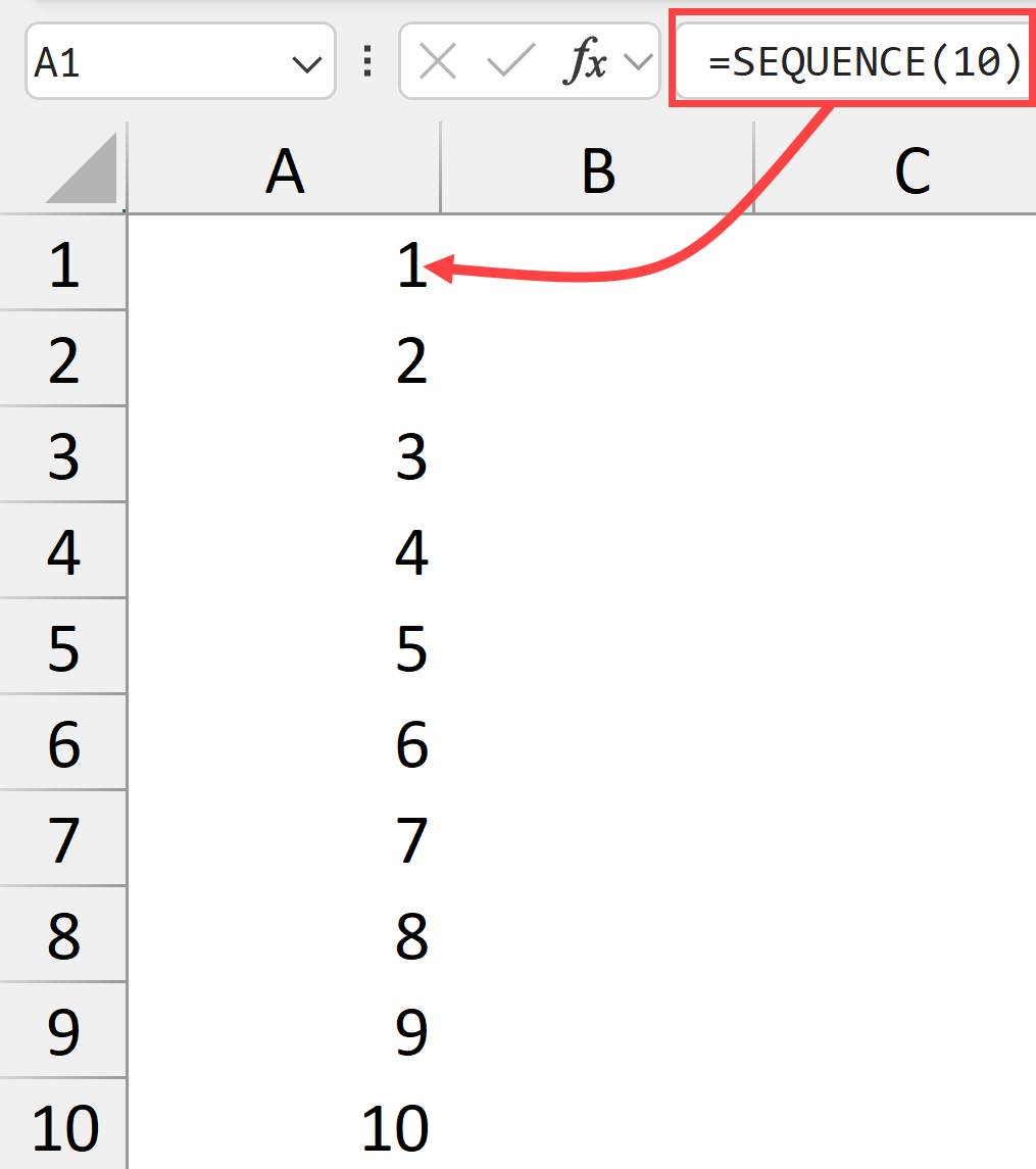
If you enter the following formula in a cell, you’ll get numbers 1 through 10 in a single column. The function always starts with 1 and increments by 1 unless you specify otherwise.
=SEQUENCE(10)
Want those numbers in a row instead? Use the below formula:
=SEQUENCE(,10)
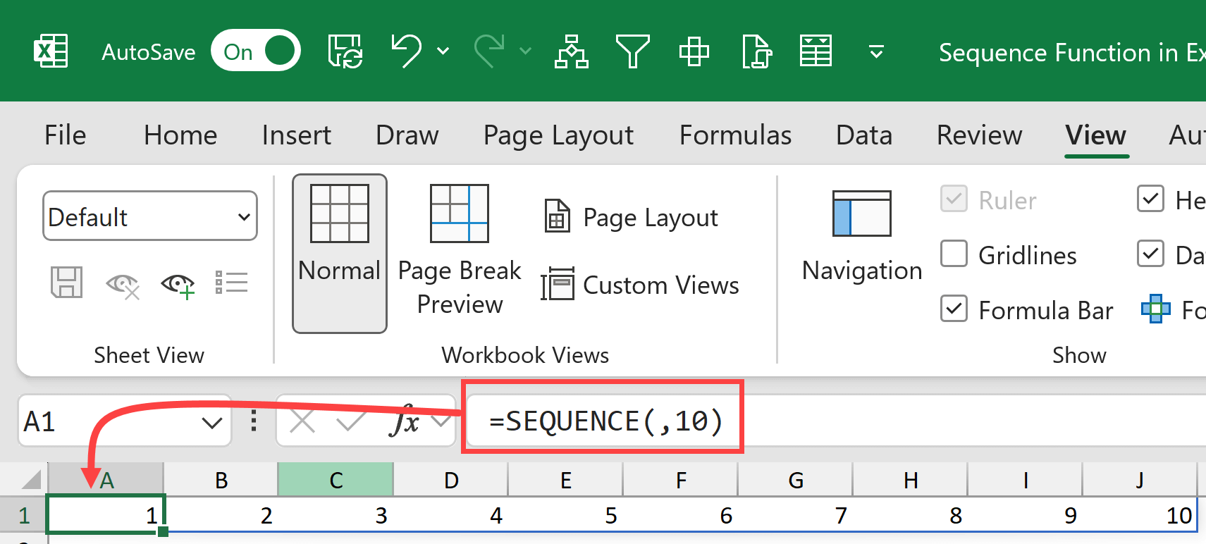
Notice how I left the first argument (rows) empty and put 10 in the columns position. This tells Excel that I do not need the 10 numbers in different rows but rather I want them in different columns, which puts them in one single row.
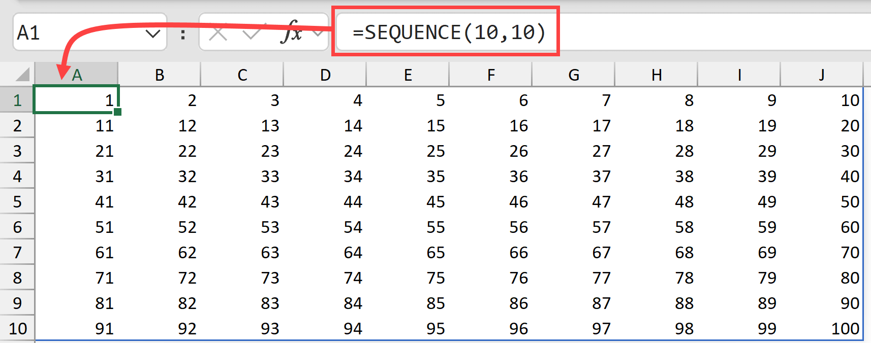
If you want to fill a grid of rows and columns that has a sequence of numbers, you can use a formula as shown below.
=SEQUENCE(10,10)
This creates a 10×10 grid where numbers increment horizontally across each row.
Pro tip: If you want the increment to happen down the column instead of across the row, wrap your SEQUENCE function in TRANSPOSE:
=TRANSPOSE(SEQUENCE(10,10))
Changing the Start Value
By default, the SEQUENCE function will start the numbering from one, but if you want, you can change the start value by specifying that in the third argument of the function.
For example, if I want the numbering to start from 5, then I can use the below formula.
=SEQUENCE(10,,5)
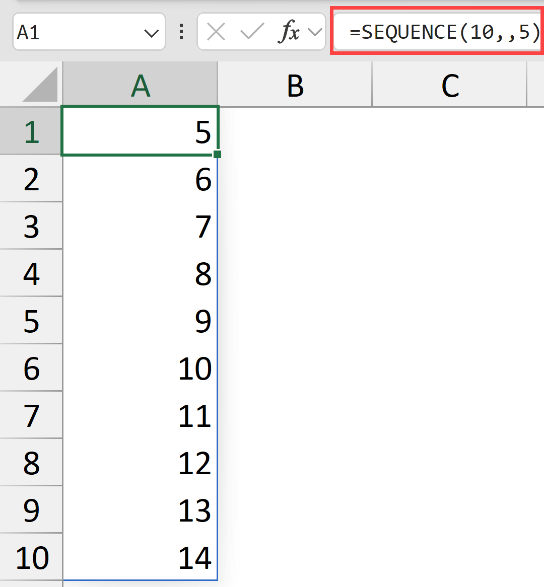
This formula gives me a sequence of 10 numbers, starting from 5 and going up to 14.
Changing the Step Value
You can also change the step value, which is the difference between each value generated by the SEQUNECE function.
By default, this value is 1. You can change this by specifying it as the fourth argument of the function.
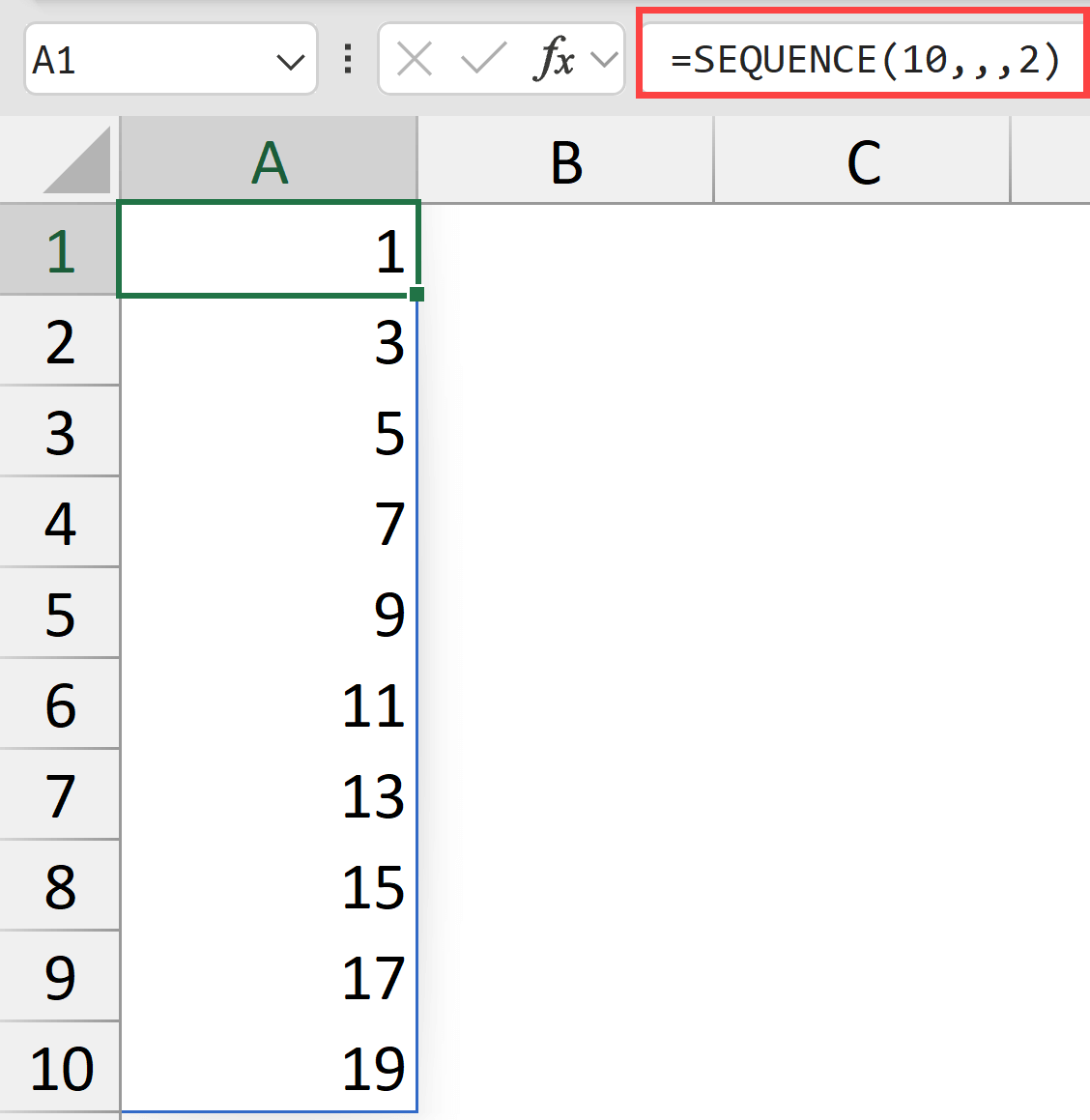
Below is the function that generates ten numbers starting from 1, where the step value is 2.
=SEQUENCE(10,,,2)
Click here to download the example file
Practical Examples of Using SEQUENCE Function in Excel
Now let’s dive into the exciting part – practical examples that showcase the true power of the SEQUENCE function.
Example 1 – Creating Date Sequences
The most common real-life use case of using the SEQUENCE function in Excel is to generate dates.
To do this, we can combine this function with the TODAY function in Excel.
Getting Dates of 30 days starting from Today
Below is the formula that will give you a list of 30 days starting from the current date.
=SEQUENCE(30,,TODAY())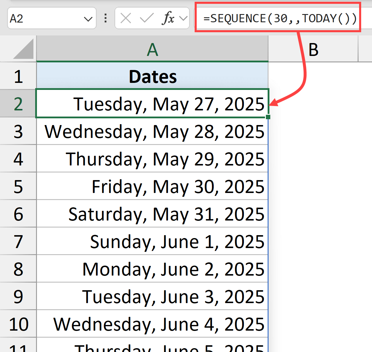
This formula creates a list of 30 consecutive dates starting from today. The beauty is that it automatically updates every day.
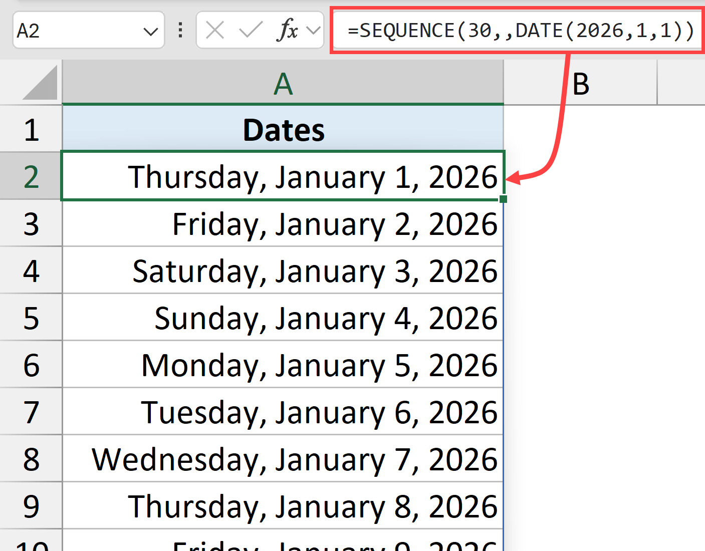
In case you want to start from a specific date, you can replace the TODAY function with the DATE function where you can specify the day, month, and year values.
For example, if I want a series of 30 dates starting from 1st January 2026, then I can use the below function.
=SEQUENCE(30,,DATE(2026,1,1))
Getting Alternate Dates
To get a sequence of alternate dates, you can specify the step value as 2.
This would ensure that there is a gap of two days in between every date returned by the SEQUENCE function.
=SEQUENCE(30,,TODAY(),2)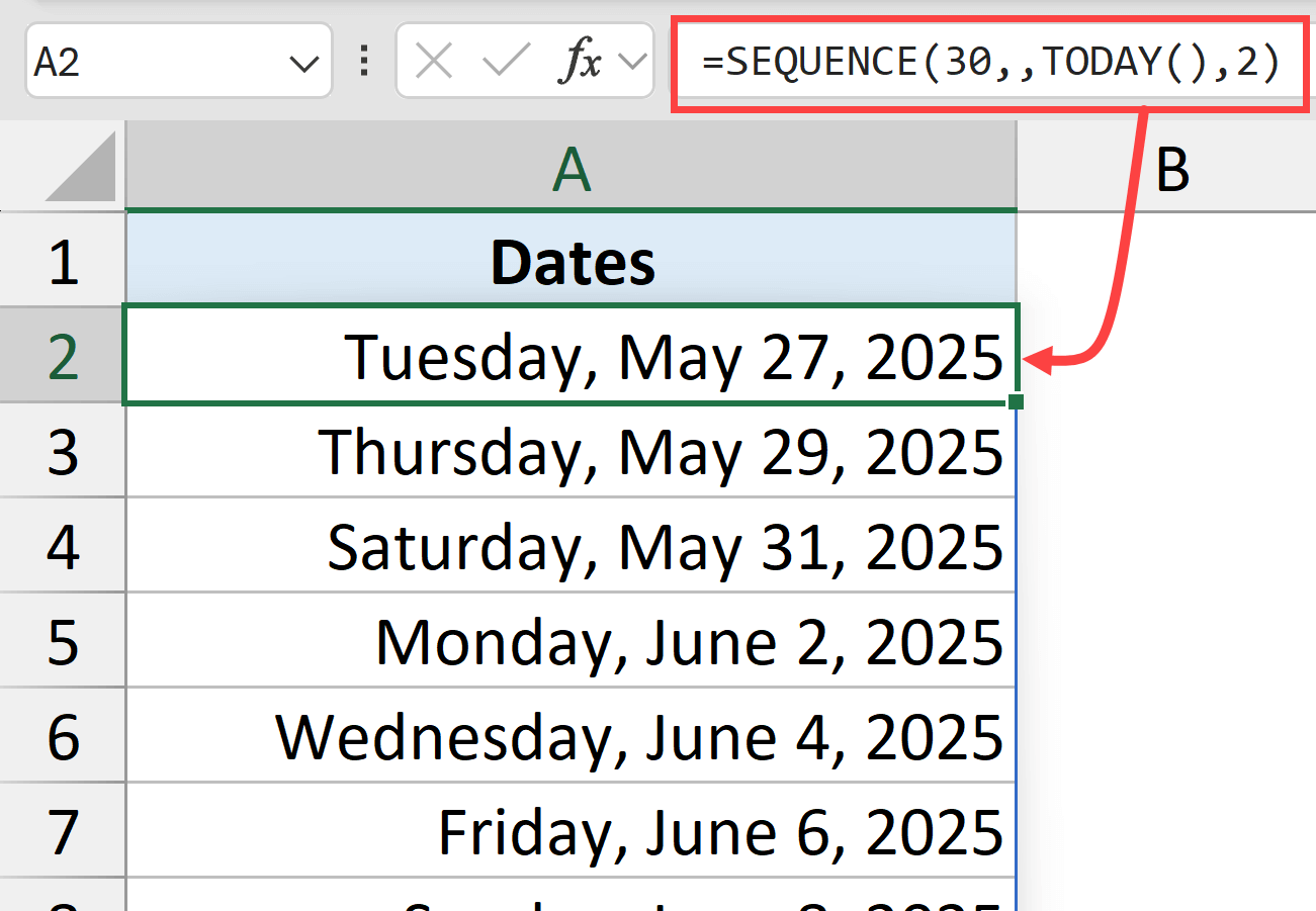
Repeating Every Date Given Number of Times
If you want to repeat dates, then you can again use the step value which is a fraction – 1/n, where n is number of times you want to repeat every date.
For example, if I want to get a list of 30 dates, where every date repeats three times, then I can use the below formula.
=ROUNDDOWN(SEQUENCE(30,,TODAY(),1/3),0)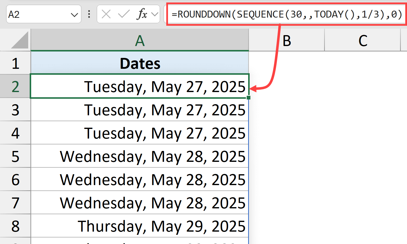
This repeats each date three times, which can be useful for scheduling scenarios.
Since dates are stored as whole numbers in the backend in Excel, when I use a step value that increments by 1 by 3, it would only become a whole number on every third date, and this is why every date is going to repeat three times.
Example 2 – Get a List of Working Days Only
Here’s where it gets really interesting.
If you want to get a list of all the working days while skipping the weekends, then you can use the below formula (considering that weekend here means Saturday and Sunday).
=WORKDAY.INTL(TODAY()-1,SEQUENCE(30),1)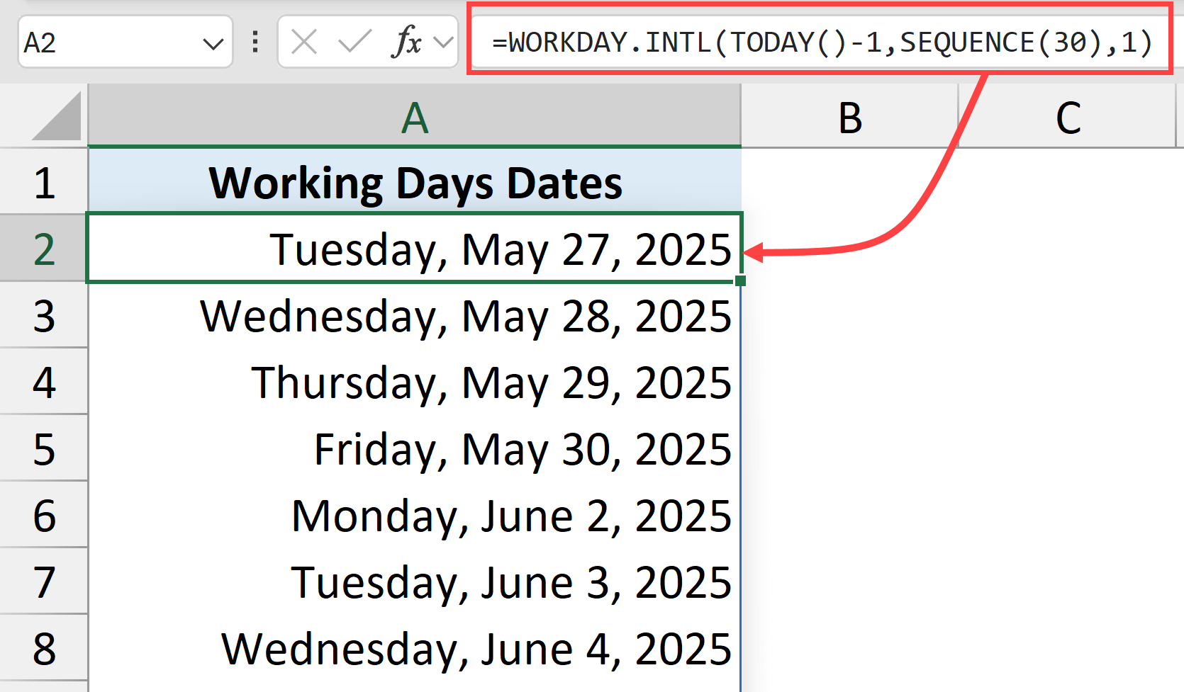
WORKDAY.INTL function in Excel gives us a working day date when we specify the start date and the number of days after the start date.
In the above example, instead of giving it one date as the second argument, I gave it SEQUNECE(30), which would generate a list of 30 numbers ({1,2,3…..30}).
So, instead of giving me the result as one single date, it would give me a list of 30 dates starting from today, ensuring that these are all working days that do not include Saturdays and Sundays.
The 1 as the last argument means that the weekend days would be Saturday and Sunday. If you want any other day to be considered as the weekend day, then you can choose from many options available in the drop-down for the last argument.
Now, what if I have a list of holidays and I want to ensure that the dates that are given to me do not include weekend days as well as any of the holidays.
Thankfully, that can also be taken care of by the WORKDAY.INTL function.
Below is the formula that would give me a list of 30 days starting from today that does not include weekend days and also does not include holidays that are listed in the last argument which is E2:E10.
=WORKDAY.INTL(TODAY()-1,SEQUENCE(30),1,E2:E10)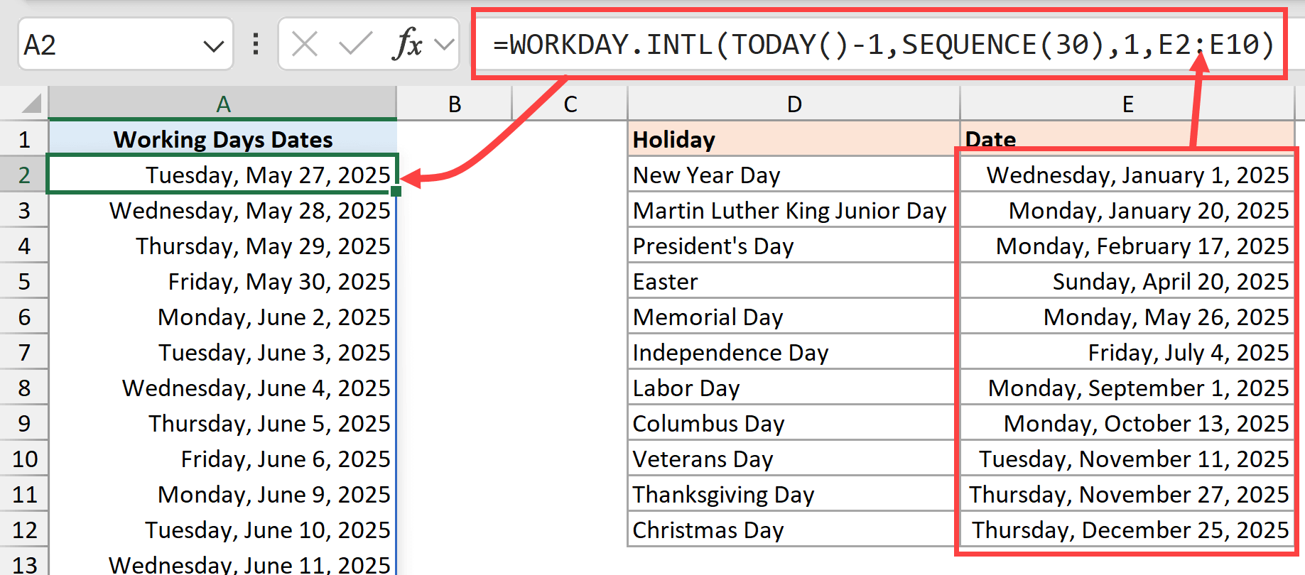
Example 3 – Custom Working Days (Tuesdays and Thursdays Only)
If you want a list of dates that only include specific weekdays, such as only Mondays or only Tuesdays and Thursdays, then that can also be done using the WORKDAY.INTL function along with the SEQUENCE function.
Below is the formula that will give me a list of 30 days starting from today that only include Tuesdays and Thursdays.
=WORKDAY.INTL(TODAY()-1,SEQUENCE(30),"1010111")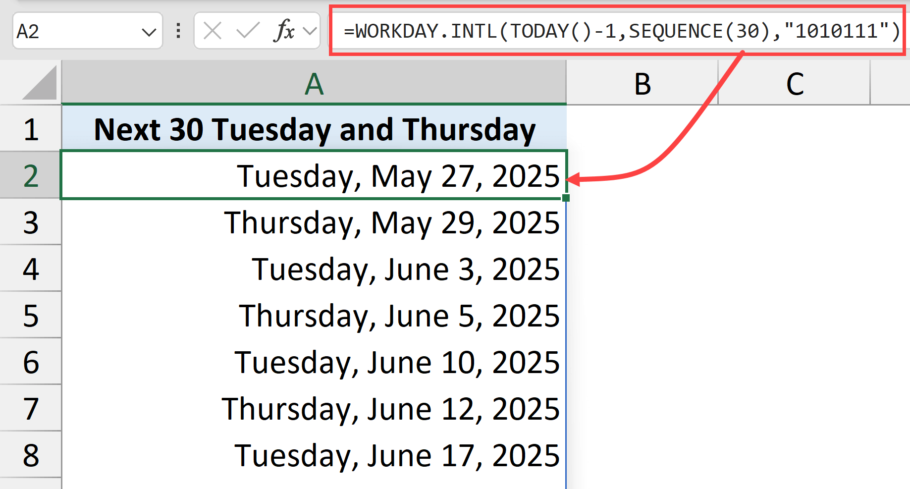
The trick here is in the last argument, where we have manually specified which days are working days and which days are non-working days.
The seven-digit string represents each day of the week (Sunday through Saturday), where 1 = non-working day and 0 = working day. So “1010111” gives you only Tuesdays and Thursdays.
4. Time Slot Generation
Below is the formula that would generate a list of time values with an interval of 30 minutes between them starting from 8 AM.
=SEQUENCE(30,,TIME(8,0,0),TIME(0,30,0))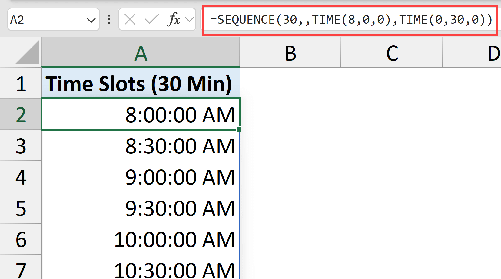
Just format the cells as time, and you have an instant schedule.
5. Extract Every Nth Row
You can use the sequence function within the filter function to extract every second or third or fourth record from a dataset.
Below I have a data set from which I want to extract every third record.
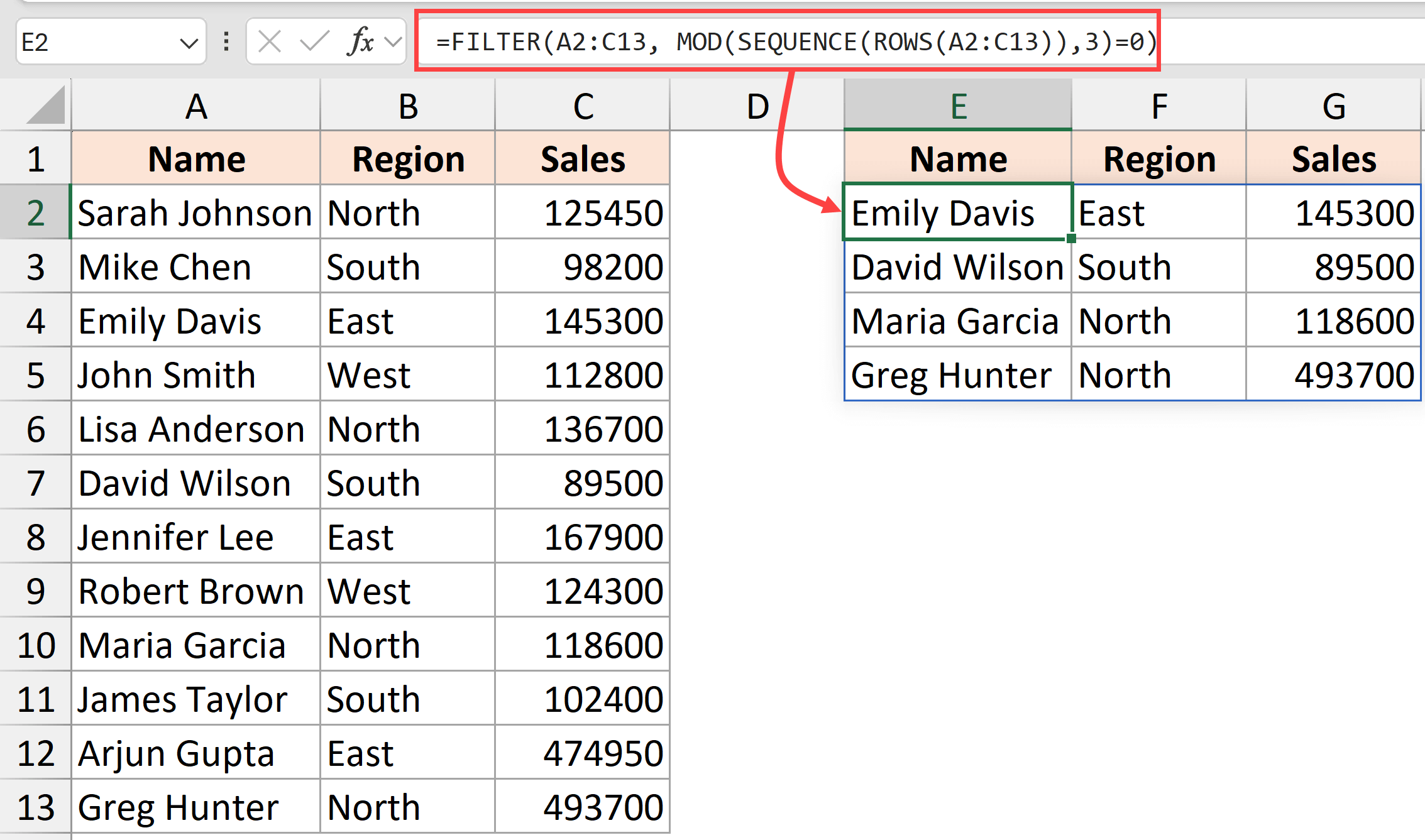
Here is the formula that will do this.
=FILTER(A2:A20,MOD(SEQUENCE(ROWS(A2:A20)),3)=0)This formula:
- Uses SEQUENCE to create numbers matching your data range
- Applies MOD function get an array of trues and falses where every third value is true.
- Uses FILTER function to extract only those records
Change the 3 to any number to extract the records with that interval.
Click here to download the example file
6. Sum of Top N Values
Below I have a dataset and I want to get the sum of top three values from the sales column.
Here is the formula that will do this.
=SUM(LARGE(B2:B20,SEQUENCE(3)))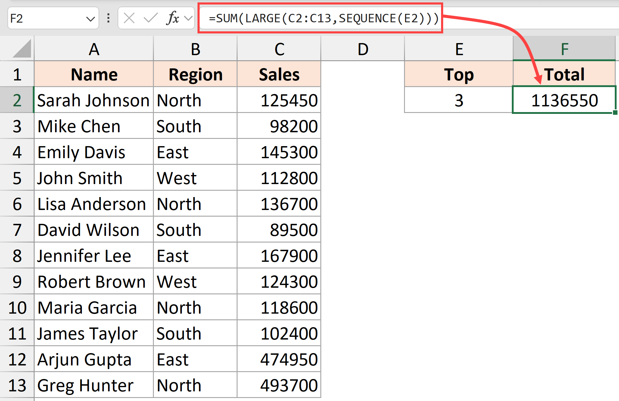
The above formula uses the LARGE function to extract the three largest values from the sales column. While the LARGE function is made to extract only one values, I have used the SEQUENCE(3) that returns a list of three numbers – {1,2,3}.
This makes the LARGE function to return the three largest values from the column. And then the SUM function is used to add these three values and give us the sum.
You can change 3 to any number and the formula will give you the sum of that many values.
7. Repeat Data Patterns
If you have a list of items or list of names and you want to repeat them any given number of times, I’ll show you how to do that using a formula that includes the SEQUENCE function.
Below I have this dataset of team names and I want to repeat these team names five times.
Here is the formula that will do that.
=INDEX(A2:A6,MOD(SEQUENCE(COUNTA(A2:A6)*5,0),COUNTA(A2:A6))+1)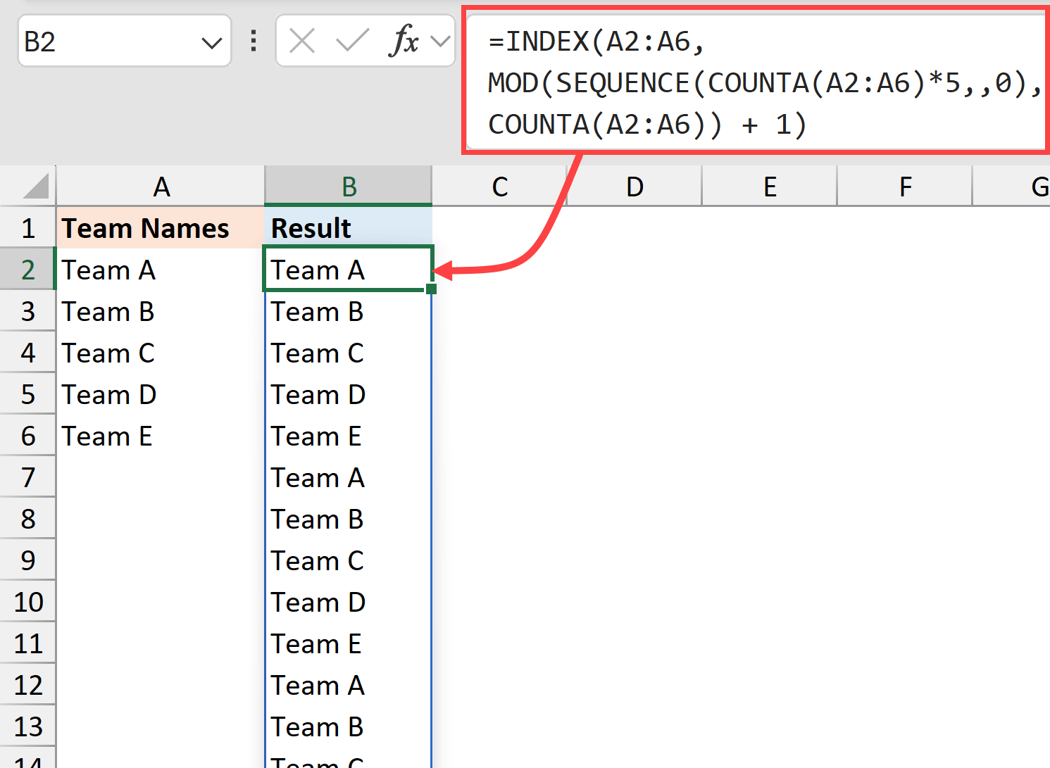
This formula:
- Counts your team names using COUNTA(A2:A6)
- Multiplies by how many times you want to repeat (5 in this example)
- Uses MOD to create the repeating pattern
- Uses INDEX retrieves the actual team names
Also read: Repeat Rows N Times in Excel
8. Dynamic Calendar Creation
Here’s the crown jewel – a complete calendar created with one formula using SEQUENCE at its core.
Below is the formula that will do that.
=LET(
    monthFirstDay, DATE(YEAR(B1),MONTH(B1),1),
    startDayShift, WEEKDAY(monthFirstDay,2)-1,
    startDateCalendar, monthFirstDay-startDayShift,
    SEQUENCE(6,7,startDateCalendar,1)
)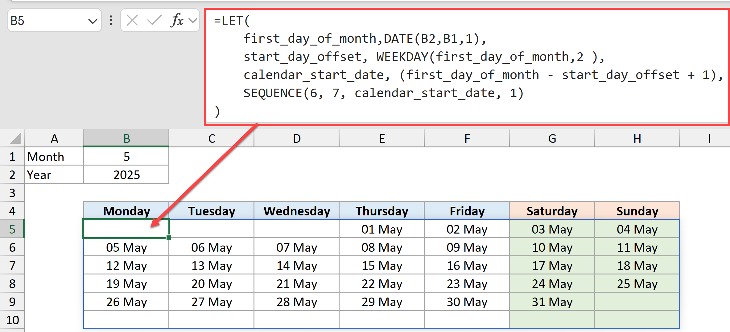
In the above formula, you have to provide the year and the month value, which is then used to create the entire calendar.
Now this would be very difficult to do without the sequence function because the sequence function allows us to quickly create a grid of six rows and seven columns and then also allows us to specify the start date for the calendar.
Some Tips When Using the SEQUENCE Function for Maximum Impact
- Combine with other functions: SEQUENCE rarely works alone. Its power comes from combination with FILTER, INDEX, WORKDAY.INTL, and others.
- Think in arrays: Remember that SEQUENCE creates arrays, so pair it with functions that can handle arrays.
- Leverage the step parameter: Don’t overlook the step parameter – it’s incredibly versatile for creating patterns and intervals.
Start experimenting with these examples, and you’ll quickly discover that the SEQUENCE function is an indispensable tool in your Excel arsenal.
The beauty lies not just in what it does, but in how it enables other functions to perform at their best.
I hope you found this article helpful. In case you have any comments or feedback, do let me know in the comment section.
Other Excel articles you may also like:


