
Thanks to some easy-to-use financial functions in Excel, it’s pretty easy to create a loan amortization schedule in Excel.
In this article, I will show you how to create a simple loan amortization schedule, when you input the details (such as the principal amount, interest rate, and duration) in some cells, it instantly generates the entire schedule for you.
I will also show you how to make a template where you can make pre-payments and it adjusts the loan amount or the loan duration accordingly.
Creating a Simple Loan Amortization Schedule in Excel
To create a simple loan amortization schedule in Excel, we need to have a place where we can enter the input data (such as the loan principal amount, the rate of interest, and the total number of periods).
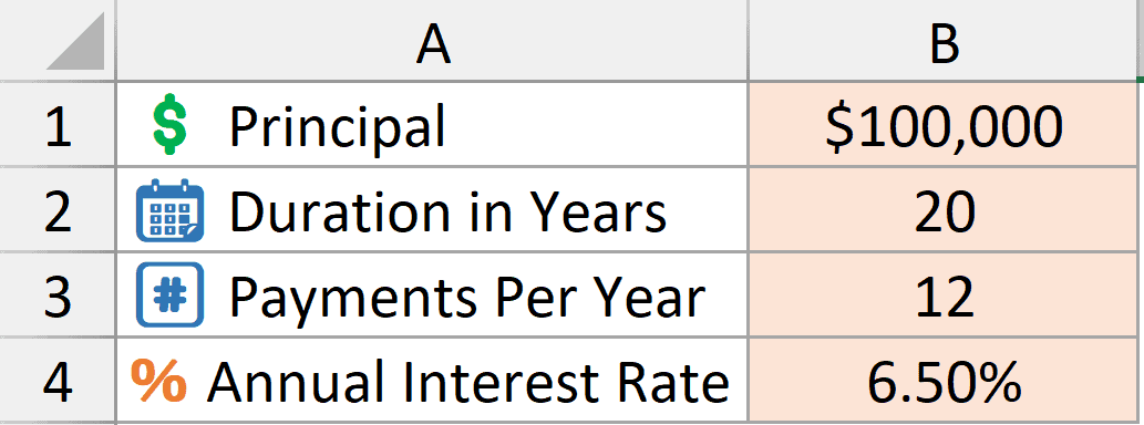
I have the input cells in column B where you can input the following data:
- Principal amount in cell B1 – this is the total loan amount for which we are creating the amortization schedule. In this example, I’m using $100,000
- Duration (in years) in cell B2 – this is the total duration of the loan in years. In this example, I am using 20 years as the loan/mortgage duration.
- Number of Payments per year in cell B3 – this is the total number of payments you’ll be making in a year. If these are monthly payments, enter 12. If it’s weekly payment, enter 52. In this example, I’ll use 12 payments per year.
- Annual Interest Rate in cell B4 – this is the annual rate of interest for the loan repayment. In this example, I am using 6.5% as annual interest rate
Once you have entered these details as inputs, we are ready to construct the amortization schedule (also called the Loan Repayment Schedule).
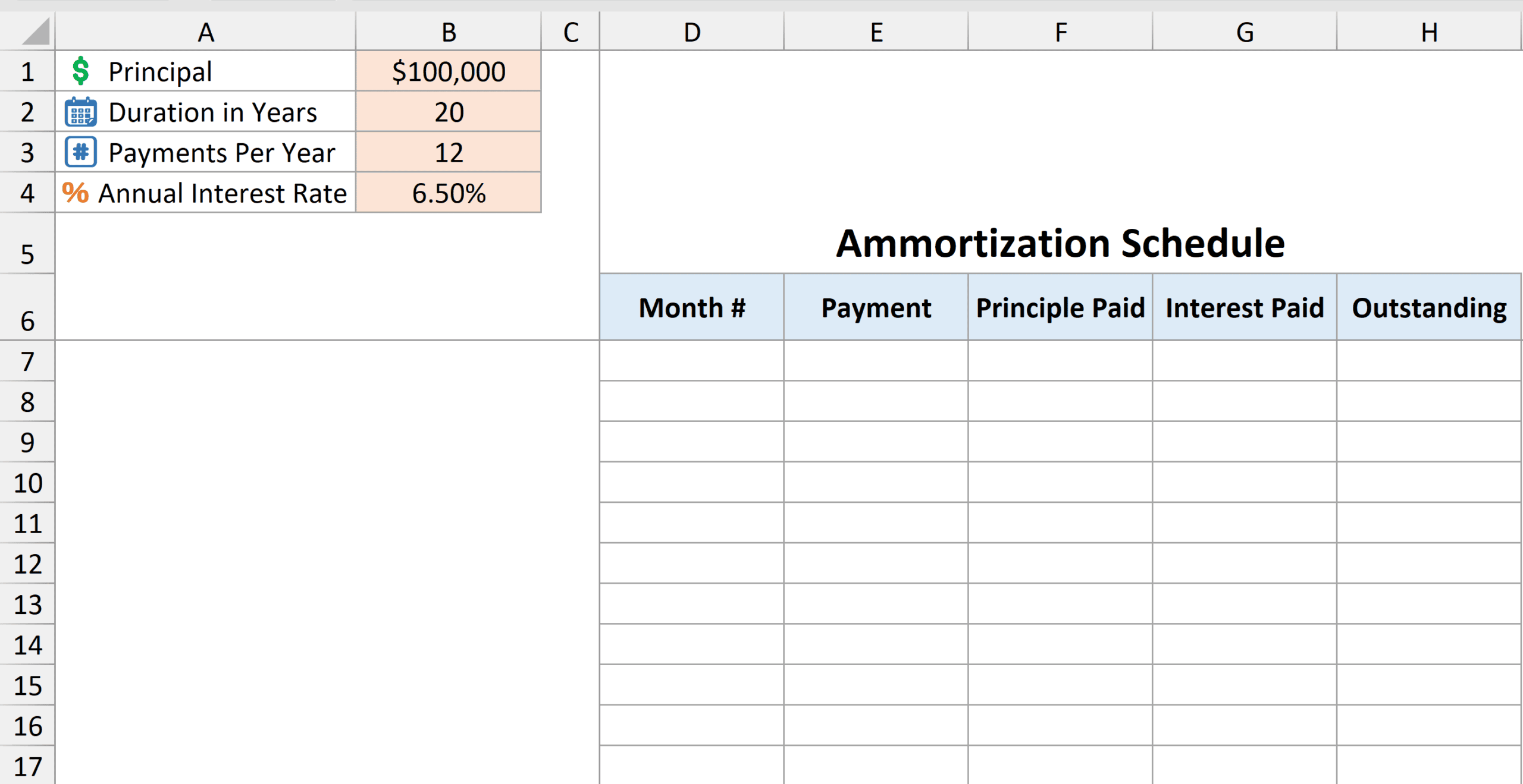
Below is the template I have created for the schedule where I will be entering formulas to create the schedule in these five columns.
Getting the Month Numbers
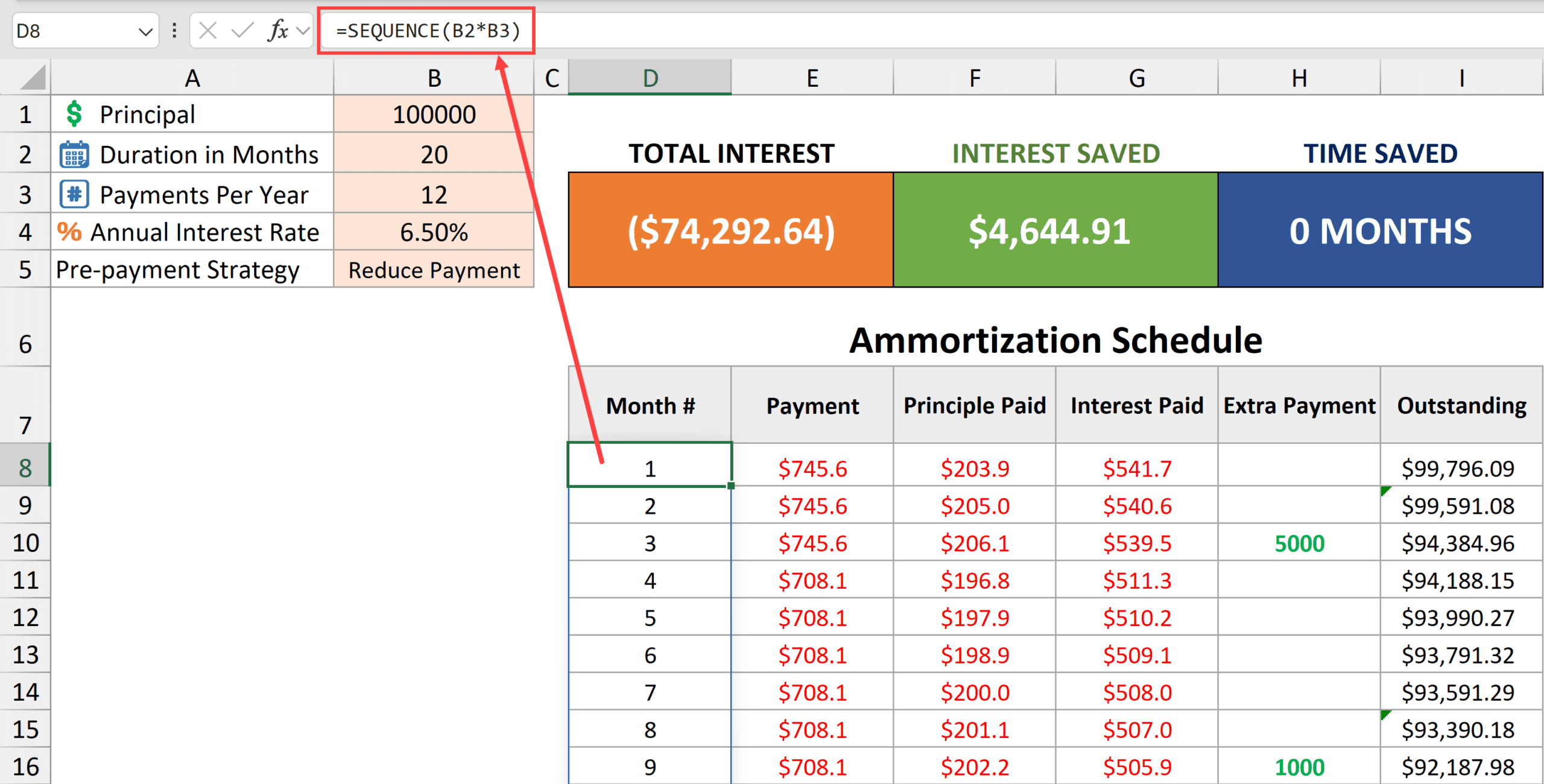
Below is the sequence function that will give me a sequence of month numbers
=SEQUENCE(B2*B3)
SEQUENCE function takes the number of years value from cell B2 and multiplies it with the payments per year value in cell B3 to create a sequence of numbers that runs down the column.
Calculating the monthly payment
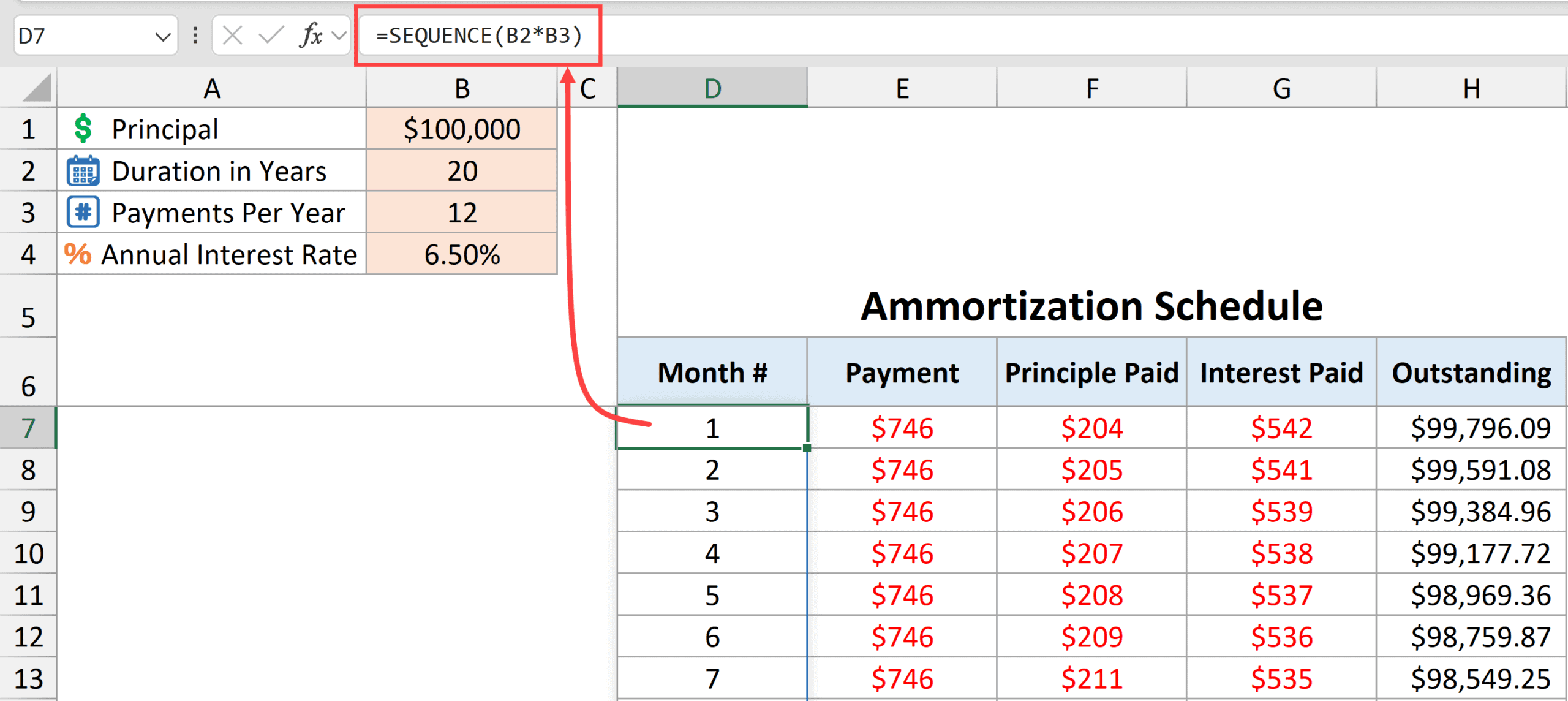
Below is the formula used to calculate the monthly payment.
=PMT($B$4/$B$3,$B$2*$B$3,$B$1)
The above PMT function would give us the monthly payment that needs to be made each month.
Enter this formula in cell E6 and then drag it down for all the cells in the column (till you have all the month numbers you need in the schedule).
It takes the following arguments:
- $B$4/$B$3 – this is the interest rate to be used. Since we have the annual interest rate in cell B4, I have divided by the value in cell B3 to get the interest rate to be used for our payment frequency (monthly in this case).
- $B$2*$B$3 – this is the total number of periods for which the loan has to be repaid. In this example, it’s 240 (20*12).
- $B$1 – this is the present value of the loan, which is $100,000.
In this scenario, since our monthly payments remain the same throughout the repayment schedule, when you drag down this formula in the column, it returns the same value.
Note that I’ve used a $ symbol in the cell reference to make them absolute. This way these cell references won’t change when I copy the formula down. If I don’t use the $ symbol in the cell references, these cell references would become relative and change when I copy the formula down.
Principal paid in each monthly payment
To calculate the principal paid every month, you can use the below PPMT formula (where PPMT stands for Principal Payment).
=PPMT($B$4/$B$3,D7,$B$2*$B$3,$B$1)
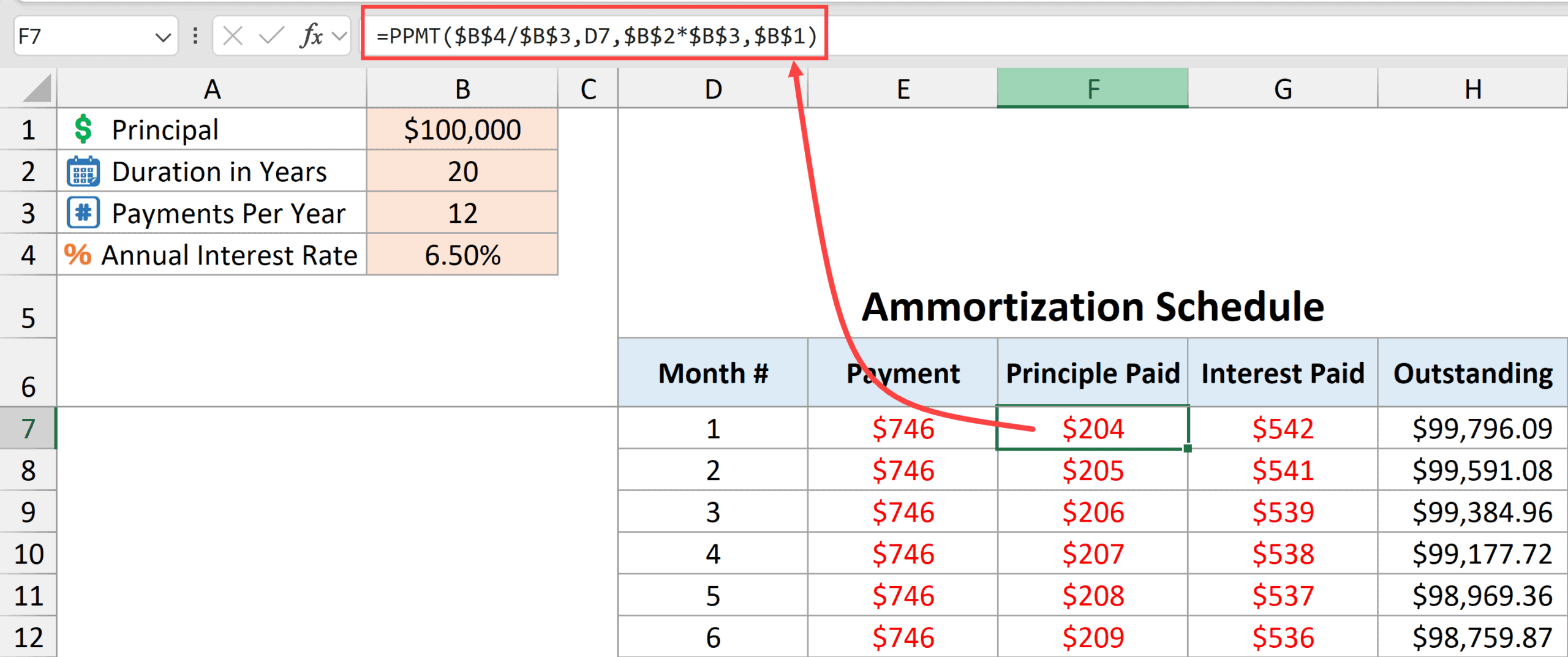
The above formula uses the following arguments:
- $B$4/$B$3 – this gives us the monthly interest rate to be used for each payment.
- D7 – this gives us the month number for which the principal amount needs to be calculated. As I copy the formula down, this value would change accordingly based on the month number (notice no $ signs in this argument).
- $B$2*$B$3 – this is the total number of periods in the entire duration of the loan repayment schedule.
- $B$1 – this is the loan amount with which we started ($100,000 in this example).
Interest paid in each monthly payment
Since I already have the principal and total payment value of each month, I can use the simple subtraction formula below to get the monthly interest payment.
=E7-F7
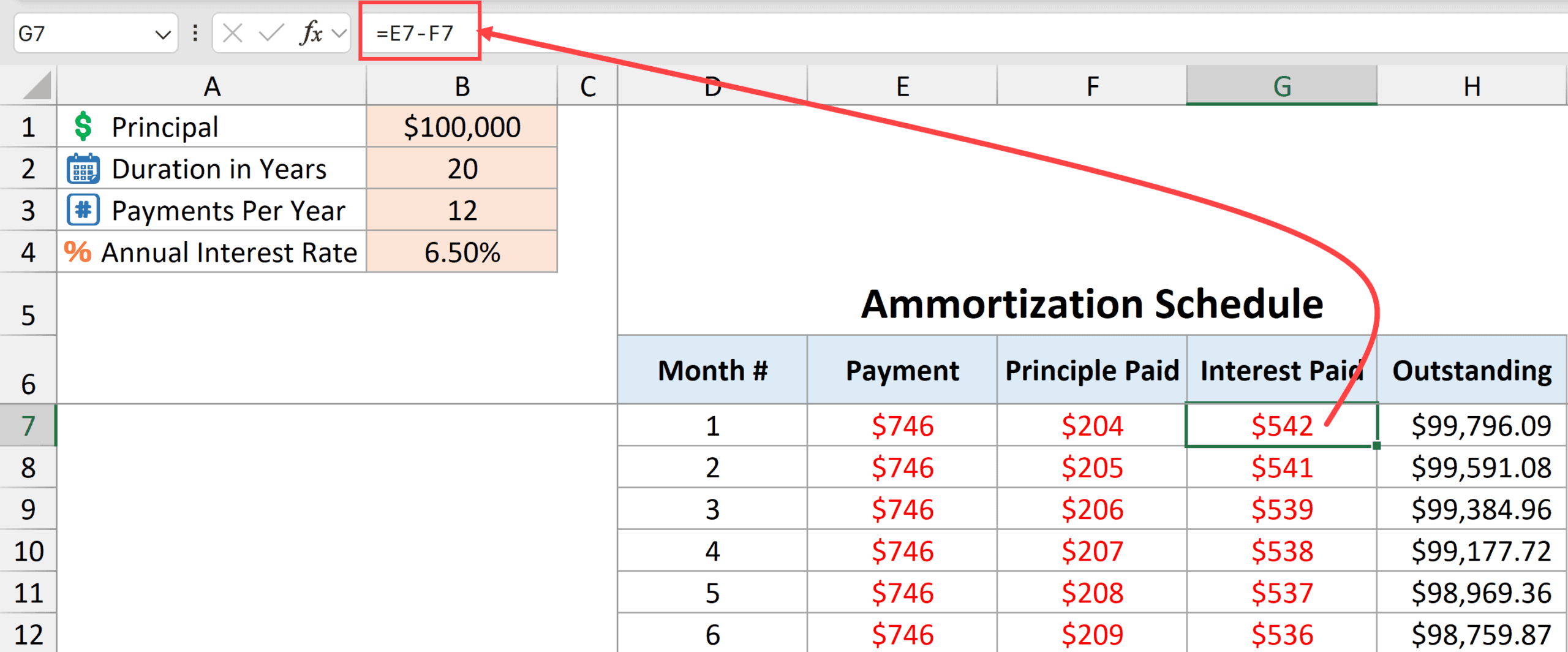
The above formula subtracts the principal part from the total payment for a given month and gives us the total interest paid in that month.
Outstanding loan at the end of each period
=$B$1+SUM($F$7:F7)
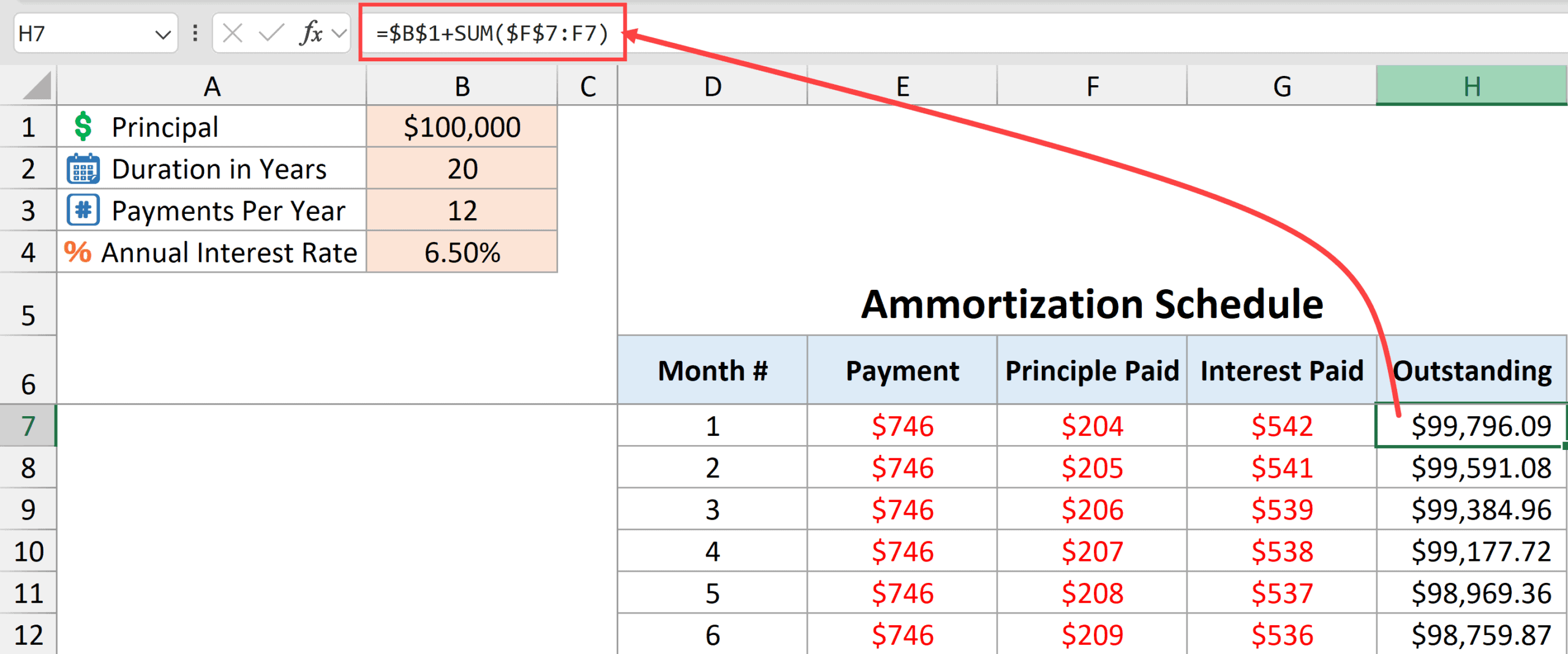
The above formula starts with the initial loan amount (in cell B1) and subtracts the principal part of the loan paid till every month.
SUM($F$7:F7) – this part of the formula gives us the cumulative principal paid for every month. And I’ve added this to the initial loan amount in cell B1 to get the remaining principal amount.
Note that SUM($F$7:F7) returns a negative value, so when I add this to cell B1, it gives us the remaining principal amount.
Calculating Total Interest Payment Over Loan Duration
It could be helpful to also show the total interest payment that needs to be done during the entire loan duration.
You can get that using the below formula.
=SUM(G7:G1000)
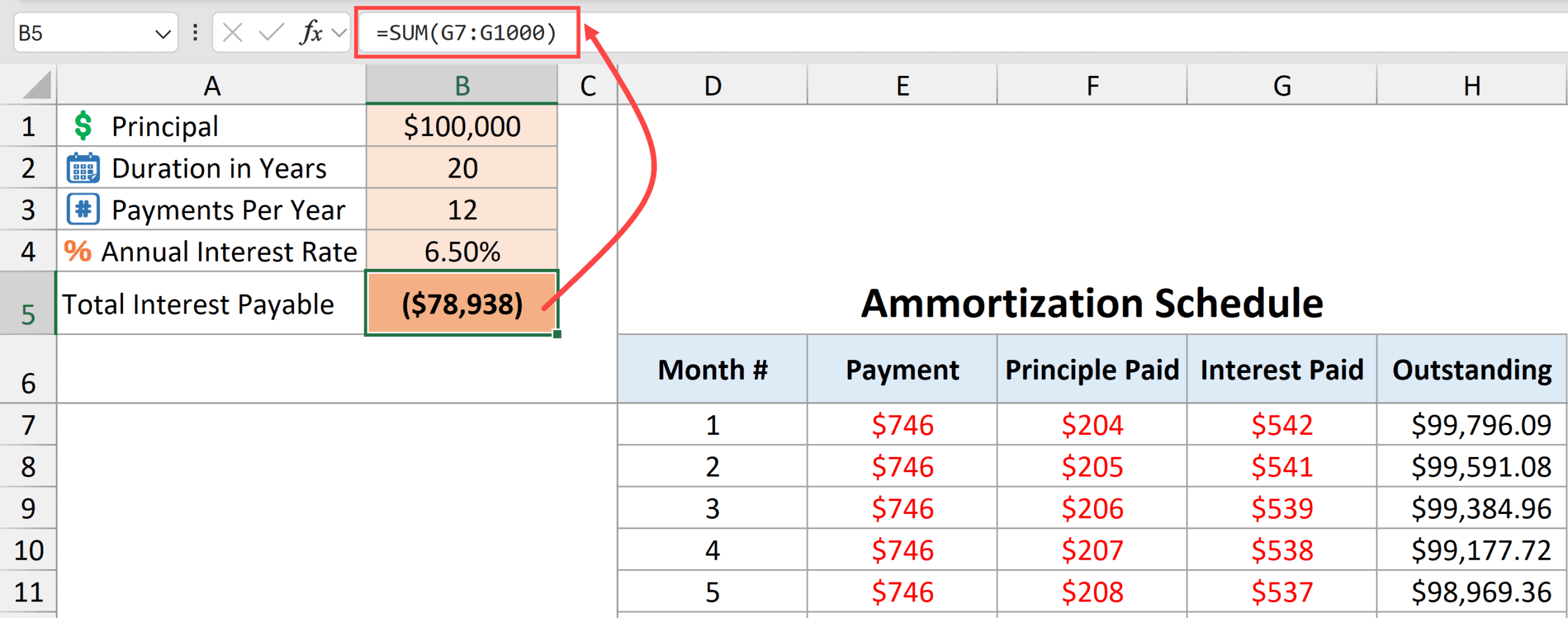
When you have applied all the formulas mentioned above, you will have a working loan amortization schedule template as shown below.
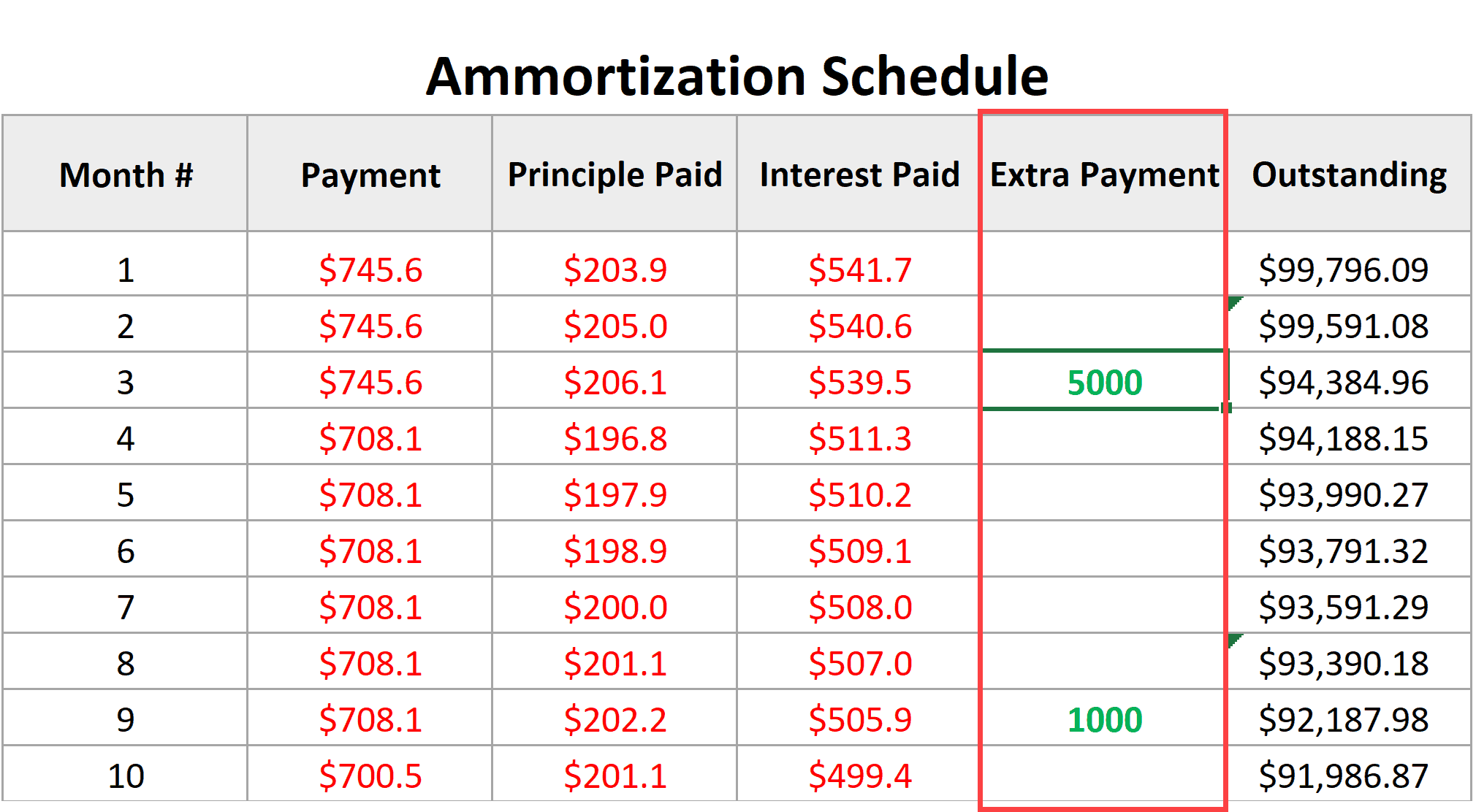
Loan Amortization Schedule With Prepayments
It is a common scenario for many people to make extra payments in some months, which can either reduce the loan term or lower the monthly payment.
In this section, I will show you how to create a template that allows you to specify extra payments within the loan repayment schedule and also choose whether you want to reduce the loan term or lower the monthly payment.
- When you reduce the loan term, the monthly payment remains the same.
- When you lower the monthly payment, the repayment duration remains the same.
First, we would have the cells where we need to provide the input for the amortization schedule.
- Enter the principal amount in cell B1. In this example, I’m using $100,000
- Enter the duration in years in cell B2 – In this example, I’m using 20 years.
- Enter the total number of payments per year in cell B3. If these are monthly payments, enter 12. If it’s weekly payment, enter 52. In this example, I’ll use 12 payments per year.
- Enter the annual interest rate in cell B4. In this example, I am using 6.5% as annual interest rate
- Select one of the options (Reduce Term or Reduce Payment) from the drop-down in cell B5. For this example, I’ll choose Reduce Payment option
Now let’s use some formulas to create a dynamic loan amortization schedule template.
Getting the Month Numbers
Below is the sequence function that will give me a sequence of month numbers
=SEQUENCE(B2*B3)
SEQUENCE function takes the number of years value from cell B2 and multiplies it with the payments per year value in cell B3 to create a sequence of numbers that runs down the column.
Calculating the monthly payment
Below is the formula that will calculate the monthly payment based on the chosen scenario (which could be a reduced term or reduced payment).
=IF($B$5="Reduce Term",PMT($B$4/$B$3,$B$2*$B$3,$B$1),PMT($B$4/$B$3,$B$2*$B$3-D8+1,IF(D8=1,$B$1,I7),0))
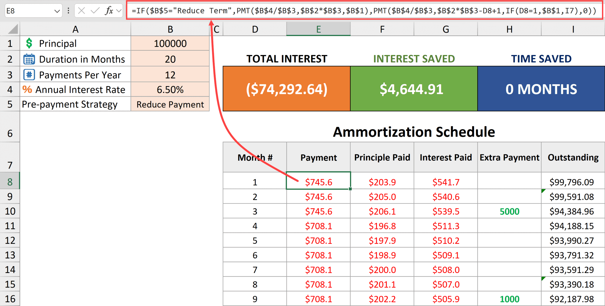
The above formula first checks the value in cell B5.
- If the value in cell B5 is “Reduce Term”, it uses the formula PMT($B$4/$B$3,$B$2*$B$3,$B$1) to give us the monthly payment
- If the value in cell B5 is “Reduce Payment”, it uses the formula PMT($B$4/$B$3,$B$2*$B$3-D8+1,IF(D8=1,$B$1,I7),0) to give the monthly payment.
Let me quickly explain both of these formulas.
PMT($B$4/$B$3,$B$2*$B$3,$B$1)
The above formula is a straight-forward PMT formula that uses the values in cells B1, B2, B3, and B4 to give us the monthly payment.
This formula is used when we have chosen the option “Reduce Term”, which means that our monthly payment is going to remain the same throughout the schedule.
PMT($B$4/$B$3,$B$2*$B$3-D8+1,IF(D8=1,$B$1,I7),0)
And the above part of the formula is used when the ‘Reduce Payment’ option is selected.
In the above PMT formula
- $B$4/$B$3 – this is the monthly rate of interest to be used.
- $B$2*$B$3-D8+1 – this changes the tenure of the loan as we copy the formula down the column. For the first cell, the tenure remains 240. As we go down each cell, the tenure goes down by 1 (so it becomes 239, then 238, then 237, and so on). The reason we need to do this is because after the pre-payment, the monthly payment needs to change. We consider each monthly payment as if it’s the first payment on a new loan that has a given duration. So, for cell E9, it would consider the payment where the duration of the loan is 239 months and the principal on which the loan is taken is in cell I8.
- IF(D8=1,$B$1,I7) – here we need to specify the outstanding loan on which the monthly payment is calculated. If it is a first month, we take the original value of the loan in cell B1, and after that, we pick up the outstanding loan value from column I.
Calculating the Principal Amount Paid Each Month
Below is the formula to calculate the principal portion that is paid with every monthly payment.
=IF($B$5="Reduce Term",IF(ABS(E8-G8)>I7,-I7,E8-G8),PPMT($B$4/$B$3,1,$B$2*$B$3-D8+1,IF(D8=1,$B$1,I7)))
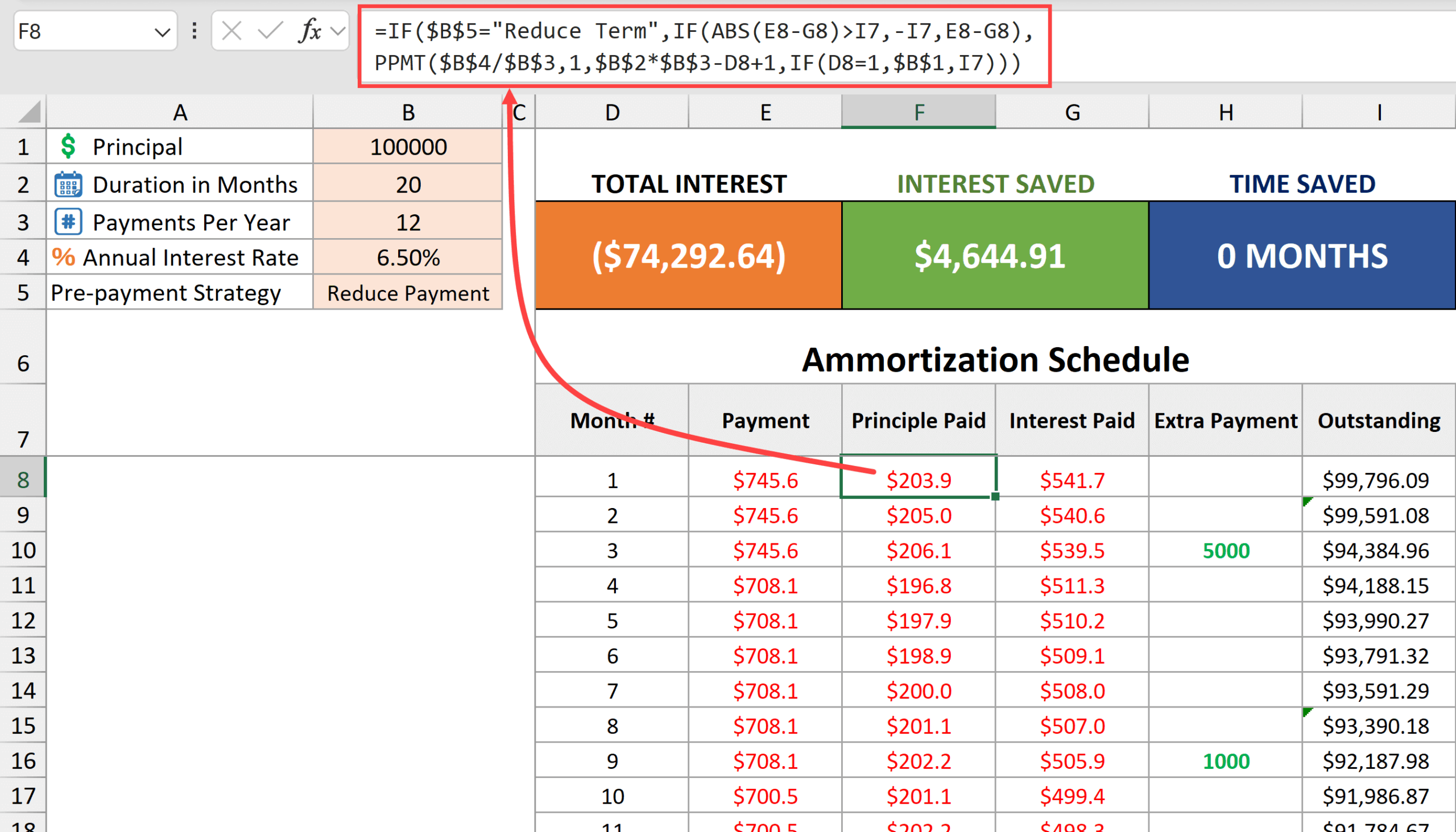
The above formula first checks the value in cell B5.
- If the value in cell B5 is “Reduce Term”, it uses the formula IF(ABS(E8-G8)>I7,-I7,E8-G8)
- If the value in cell B5 is “Reduce Payment”, it uses the formula PPMT($B$4/$B$3,1,$B$2*$B$3-D8+1,IF(D8=1,$B$1,I7))
Let me quickly explain both of these formulas.
IF(ABS(E8-G8)>I7,-I7,E8-G8)
This part of the formula is used when the ‘Reduce term’ option is selected.
It calculates the principal portion of the payment by subtracting the interest in cell G8 from the payment amount in cell E8. While I could have just used E8-G8, I have wrapped it inside an IF function to account for the month where the last payment is made. If I don’t use the IF function, then it won’t show the outstanding balance as 0.
PPMT($B$4/$B$3,1,$B$2*$B$3-D8+1,IF(D8=1,$B$1,I7))
This part of the formula is used when the ‘Reduce Payment’ option is selected.
Since with the “Reduce Payment” option, the total number of periods remains unchanged, PPMT function can be used to calculate the principal portion of the payment every month.
Calculating the Interest Portion in Monthly Payment
To calculate the interest amount in the monthly payment, I’ve used the below formula.
=IF($B$5="Reduce Term",IPMT($B$4/$B$3,1,$B$2*$B$3+1-D8,IF(D8=1,$B$1,I7)),E8-F8)
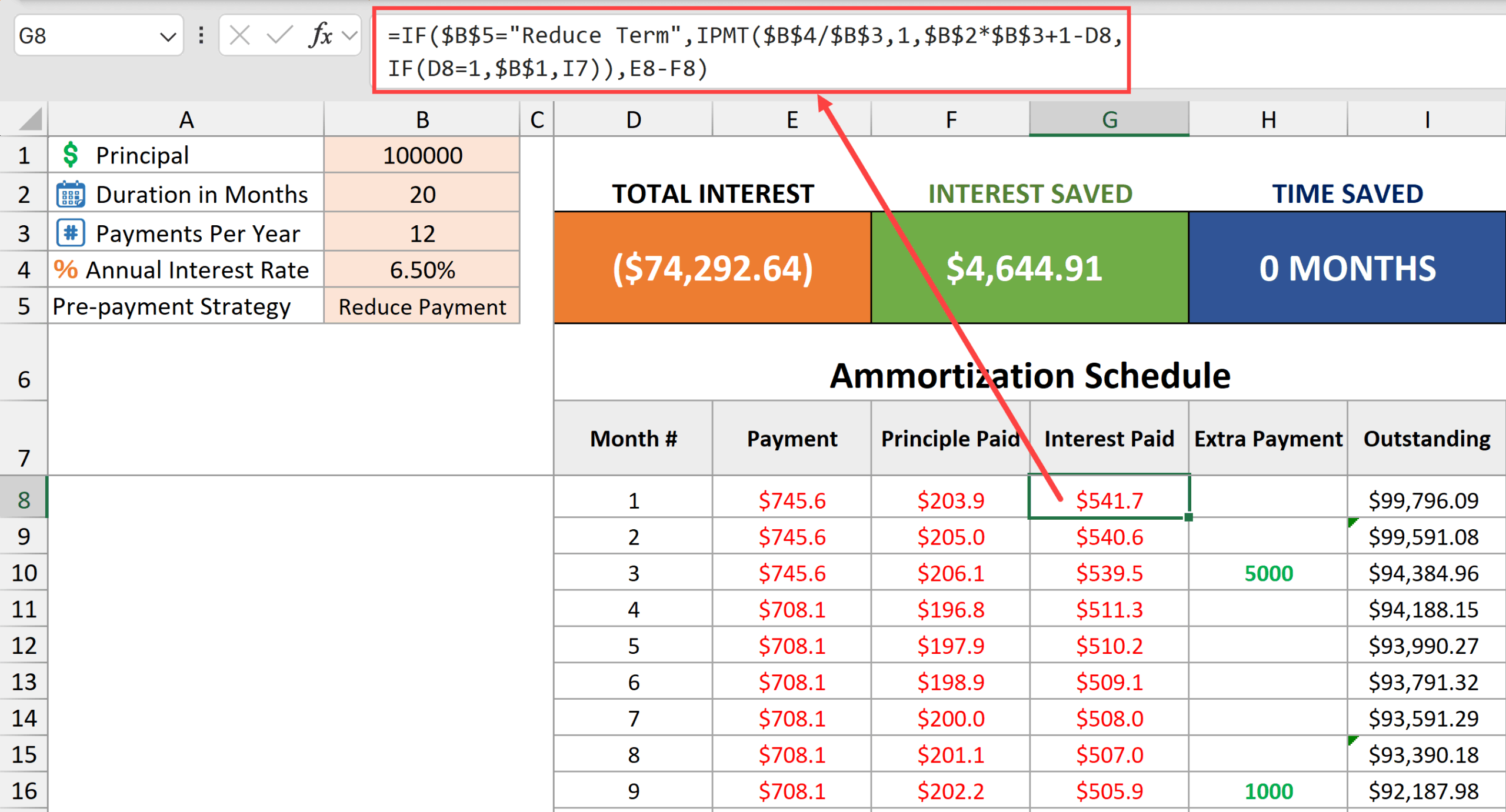
The above formula first checks the value in cell B5.
- If the value in cell B5 is “Reduce Term”, it uses the formula IPMT($B$4/$B$3,1,$B$2*$B$3+1-D8,IF(D8=1,$B$1,I7))
- If the value in cell B5 is “Reduce Payment”, it uses the formula E8-F8
Let me explain these formulas.
IPMT($B$4/$B$3,1,$B$2*$B$3+1-D8,IF(D8=1,$B$1,I7))
This part of the formula is used when the ‘Reduce term’ option is selected.
It calculates the interest payment every month by using
- $B$4/$B$3 as the monthly interest rate
- $B$2*$B$3+1-D8 as the number of period. As the formula is copied down the column, this value changes from 240 to 239 to 238 and so on.
- IF(D8=1,$B$1,I7) as the outstanding balance. For the first month, where the value in cell D8 is 1, it uses the principal amount value in cell B1 (100000) and after that it takes the outstanding balance in column I.
And in case ‘Reduce Payment’ is selected in cell B5, the following formula is used.
E8-F8
Extra Payment Entry
The template contains an empty column for extra payment value where you can manually enter the extra payment value. This value is over and above the monthly payment.
Outstanding Loan Amount
We’ll use the formula to calculate the outstanding loan amount after every month’s payment.
=$B$1+SUM($F$8:F8)-SUM($H$8:H8)
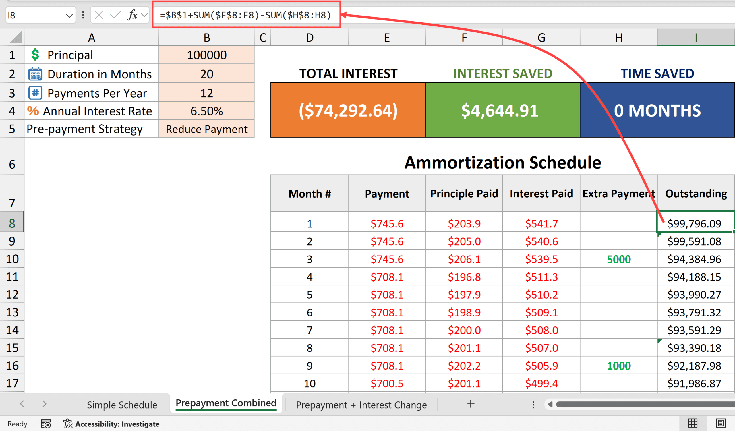
The above formula starts with the value in cell B1 (the actual loan value in the beginning) and then subtracts the principal amount that is already paid (in column F) as well as any repayment in column H.
Along with the amortization schedule, I have also provided some useful information (such as total interest, interest saved, and time saved) at the top of the template.
Here are the formulas to calculate these values.
Total Interest
=SUMIF(G8:G1001,"<0")
Interest Saved
=ABS(SUM(IPMT(B4/B3,SEQUENCE(B2*B3),B2*B3,B1))-B6)
Time Saved
=COUNTIF(G8:G1001,">=0")
Other Excel articles you may also like:


Regarding the Template- It appears the “With Prepayment” sheet incorrectly references cell I7 (Text Value) in the formulas in cells E8, F8, G8 which zeros out the “Principal Paid” (column F)? Perhaps I am missing a (manual?) data entry field somewhere?
It is not an incorrect reference; it is actually by design. For the cells in row 8, I do not want to refer to column I; instead, I want to refer to the original principal value (in cell B1). But as I drag down the formula, I do want to refer to the values in column I.
So instead of creating two different formulas, I just refer to cell I7, which is not used anyway because it ends up referring to the value in cell B1, and then when I drag down the formula, it refers to the correct cell in column I.