How to Insert a Checkbox in Excel (New In-Cell Checkboxes)

If you want to insert a checkbox in Excel, whether it’s for a to-do list, a tracker, or an interactive chart, this has now become really easy.

Earlier, Excel only had checkboxes that floated over the worksheet as separate objects, and you had to enable the Developer tab just to get to them. Excel now has a new checkbox feature where the checkbox sits inside the cell, just like any other value.

In this article, I’ll show you how to insert these new checkboxes, format them, delete them properly, and use them with formulas, conditional formatting, charts, and progress bars.

Which Excel Versions Have the New Checkboxes

The new in-cell checkboxes are only available in Microsoft 365 (Windows, Mac, and Excel for the web).

If you’re using a perpetual license version such as Excel 2024, Excel 2021, or Excel 2019, you won’t find this option. These versions only have the older Form control checkboxes, which I briefly cover at the end of this article.

So if you don’t see the Checkbox option in your Insert tab, it’s most likely because you’re not on Microsoft 365, or your version of Excel hasn’t received the update yet.

How to Insert a Checkbox in Excel

Let me show you how to insert a checkbox with an example.

Below I have a list of names in column A, and I want to insert checkboxes in column B so that I can check off each person as they complete the training.

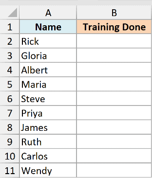
Here are the steps to insert a checkbox in Excel:

1. Select the cell (or range of cells) where you want the checkboxes. In this example, I selected B2:B11.

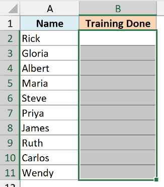
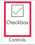
2. Click the Insert tab, and in the Controls group, click on the Checkbox icon.

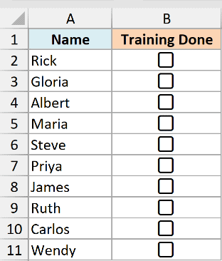
That’s it. Every cell in the selection now has a tick box that you can check or uncheck with a single click.

If you want checkboxes in multiple separate sections of your worksheet, you have two easy options:

• Hold the Ctrl key and select all the ranges where you want the checkboxes, then insert them in one go using the Insert tab.
• Or insert one checkbox, copy it (Ctrl + C), and paste it wherever you need it. A checkbox behaves like any other cell content, so copy-paste and dragging the fill handle both work just fine.

Checkboxes Are Just TRUE and FALSE Values

Behind the scenes, a checkbox is nothing but a TRUE or FALSE value in the cell. This is what makes these new checkboxes so useful.

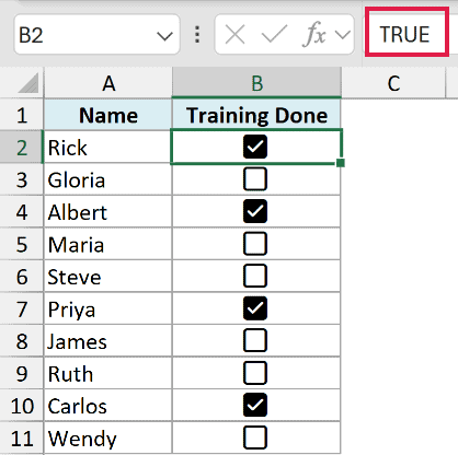
When you insert a checkbox, the cell gets the value FALSE. When you check it, the value changes to TRUE. You can see this in the formula bar when you select a cell with a checkbox.

And since the checkbox is part of the cell (not an object floating on top of it), it moves with the cell. If you move, hide, filter, or resize the cell, the checkbox goes along with it.

This TRUE/FALSE behavior is what powers everything else in this article, from counting formulas to interactive charts.

Is There a Keyboard Shortcut to Insert a Checkbox?

There is no built-in keyboard shortcut to insert a checkbox in Excel yet.

There is, however, a shortcut to check and uncheck them. Select the cell (or multiple cells) with checkboxes and press the Spacebar. This toggles the checkboxes on or off, which is a lot faster than clicking each one when you’re working with a long list.

Pro Tip: If you insert checkboxes often, right-click the Checkbox icon in the ribbon and add it to the Quick Access Toolbar. You can then insert a checkbox with Alt + the position number of the icon in the Quick Access Toolbar (for example, Alt + 4 if it’s the fourth icon).

How to Format Checkboxes (Color and Size)

Since a checkbox lives inside the cell, you format it the same way you format text in a cell.

Below I have my training list with checkboxes, and I want to make the checkboxes bigger and green.

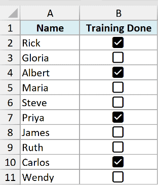
Here is how the formatting options on the Home tab affect a checkbox:

• Font color changes the color of the checkbox.
• Font size changes the size of the checkbox.
• Alignment options change where the checkbox sits within the cell (left, center, or right).

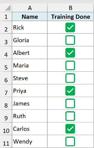
So if you want big green checkboxes for a dashboard, just select the cells, increase the font size, and change the font color to green.

How to Delete Checkboxes in Excel

Deleting checkboxes works a little differently than deleting regular cell content, so let me explain what happens.

Select the cells that have the checkboxes and press the Delete key:

• If any of the selected checkboxes are checked, the first Delete press only unchecks them all.
• Press Delete again, and the checkboxes are removed from the cells.

So if your checkboxes are all unchecked, one Delete press removes them. If some are checked, you need to press Delete twice.

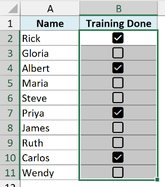
There are also two options in the Home tab (in the Clear drop-down in the Editing group) that you may find useful:

• Clear Formats removes the checkbox but keeps the TRUE or FALSE value in the cell.
• Clear All removes both the checkbox and the value, giving you a completely empty cell.

Note: When these checkboxes were first released, pressing Delete would hide the checkbox but leave it lurking in the cell, and you had to use Clear All to truly remove it. Microsoft has since fixed this, and the Delete key now removes checkboxes properly as described above.

Using Checkboxes with Formulas

Since every checkbox is just a TRUE or FALSE value, you can use regular Excel formulas to pull useful information from your checklists.

Count Checked (or Unchecked) Checkboxes

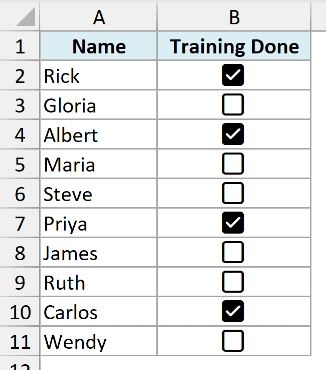
Below I have my training list, where some people have been marked as done, and I want to count how many people have completed the training.

Here is the formula that counts the checked checkboxes:

=COUNTIF(B2:B11,TRUE)

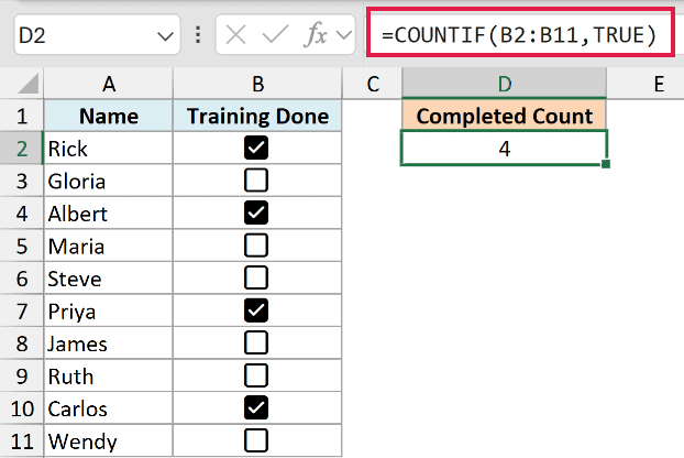
The COUNTIF function goes through the range B2:B11 and counts all the cells that have the value TRUE, which is every checked checkbox. To count the unchecked ones instead, use FALSE as the criteria.

And the count updates automatically. Check or uncheck any box, and the result changes instantly.

Calculate the Percentage of Tasks Done

You can take this one step further and calculate what percentage of the training is complete.

Here is the formula:

=COUNTIF(B2:B11,TRUE)/COUNTA(A2:A11)

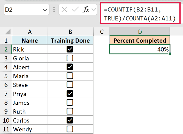
This divides the number of checked boxes by the total number of people in the list. Format the result as a percentage (Ctrl + Shift + %), and you have a live completion percentage.

Filter Records Based on the Checkbox

You can also extract records based on the state of the checkbox using the FILTER function.

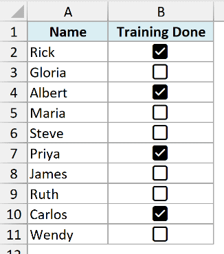
Below is the same list, and I want to get the names of all the people who have not completed the training yet.

Here is the formula:

=FILTER(A2:A11,B2:B11=FALSE)

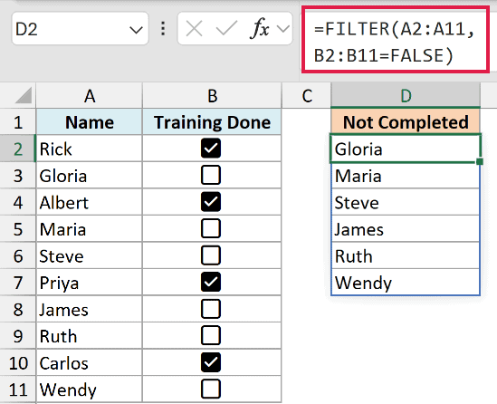
Enter this formula in a cell, and it spills the names of everyone whose checkbox is unchecked. The result is dynamic, so when you check someone’s box, their name automatically disappears from this list.

To get the list of people who have completed the training, change FALSE to TRUE in the formula.

Note: The FILTER function is available in Excel 365 and Excel 2021 or later versions. Since the new checkboxes are only in Excel 365 anyway, you’ll have it.

Highlight Rows Based on the Checkbox (Conditional Formatting)

One of my favorite ways to use checkboxes is to make the whole row react when a box is checked. Let me show you how to highlight the row in green and strike through the name when the checkbox is checked.

Below I have the training list with checkboxes in column B.

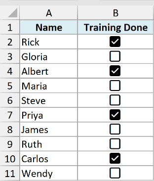
Here are the steps to set this up:

1. Select the range that has the data and the checkboxes (A2:B11 in this example).

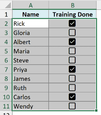
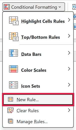
2. Click the Home tab, then Conditional Formatting, and then New Rule.

3. In the New Formatting Rule dialog box, select the option “Use a formula to determine which cells to format”.

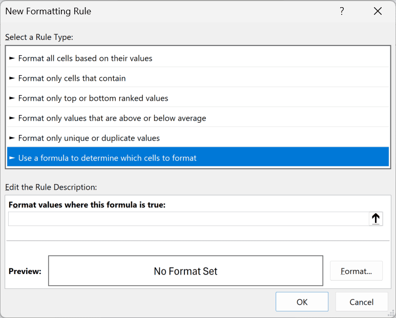
4. In the formula field, enter =$B2

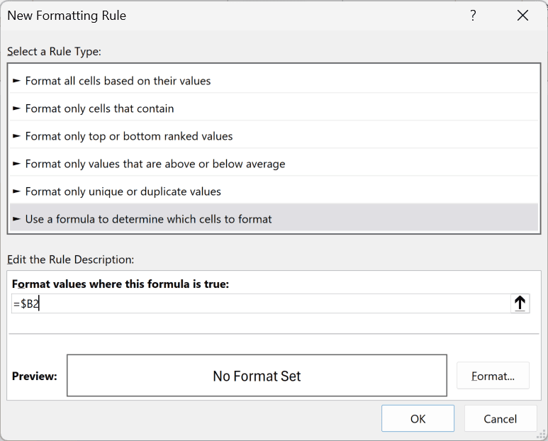
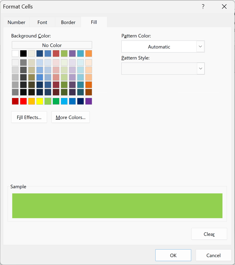
5. Click the Format button, select a green fill color in the Fill tab, check the Strikethrough option in the Font tab, and click OK.

6. Click OK to close the New Formatting Rule dialog box.

Now, as soon as you check any checkbox, that entire row gets the green color and the name gets crossed off.

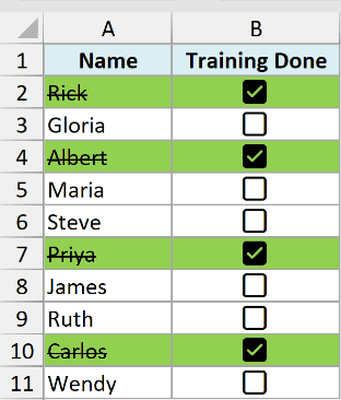
How does this work? The formula =$B2 returns the value in column B for each row, which is the TRUE or FALSE value of the checkbox. Conditional formatting applies the format wherever the formula returns TRUE, so checked rows get formatted.

And since checked names get a strikethrough format, your list reads like a real checklist, with completed items crossed off.

The dollar sign before B locks the column, so even when Excel evaluates a cell in column A, it still looks at the checkbox in column B of that same row.

Create an Interactive Chart Using Checkboxes

Now let me show you something a bit more advanced, an interactive chart where checkboxes control which data series show up.

Below I have the yearly sales data for three products (Laptops, Printers, and Monitors), and above the data I have one checkbox for each product.

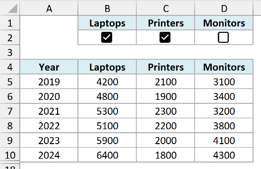
The idea is simple. Instead of plotting the original data, I use the IF function to create a helper table that only shows a product’s numbers when its checkbox is checked. The chart is then based on this helper table.

Here is the formula I use in the first cell of the helper table (cell B12):

=IF(B$2,B5,NA())

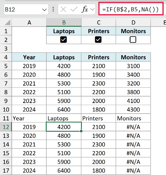
Copy this formula across all the cells of the helper table. Here is how it works:

• B$2 refers to the checkbox of that product. If it’s checked (TRUE), the formula returns the sales value from the original table.
• If the checkbox is unchecked (FALSE), the formula returns the #N/A error, and Excel simply doesn’t plot #N/A values on a chart.
• The dollar sign locks row 2 (the checkbox row), so the reference keeps pointing at the checkboxes when you copy the formula down. The column stays relative, so each product looks at its own checkbox.

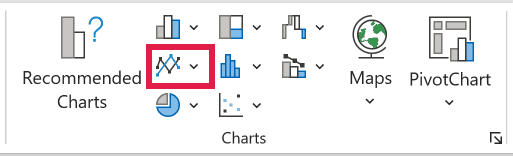
Now select the helper table, click the Insert tab, and insert a line chart.

That’s it. Check or uncheck a product’s checkbox, and its line appears or disappears from the chart instantly.

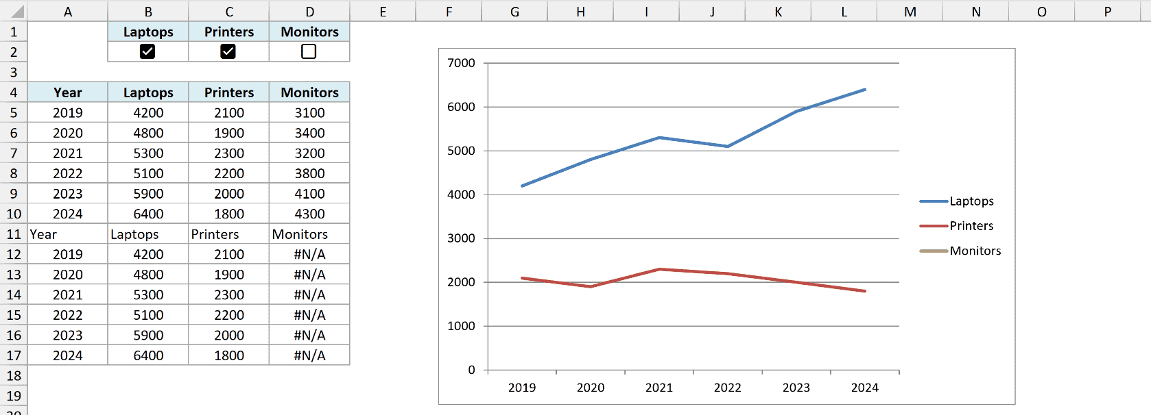
This is a great trick for dashboards, where you want to let people choose what they see instead of cramming everything into one crowded chart.

Create a Progress Bar Using Checkboxes

You can also combine checkboxes with conditional formatting to build a progress bar that fills up as you check off tasks.

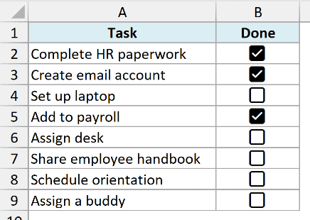
Below I have a list of tasks for onboarding a new employee, with a checkbox against each task, and I want a progress bar that shows how much of the onboarding is done.

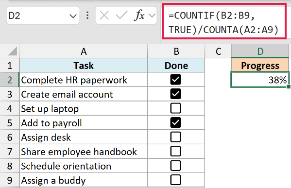
First, I calculate the percentage of tasks done. Here is the formula (I’ve entered it in cell D2):

=COUNTIF(B2:B9,TRUE)/COUNTA(A2:A9)

Now let’s turn this percentage into a progress bar:

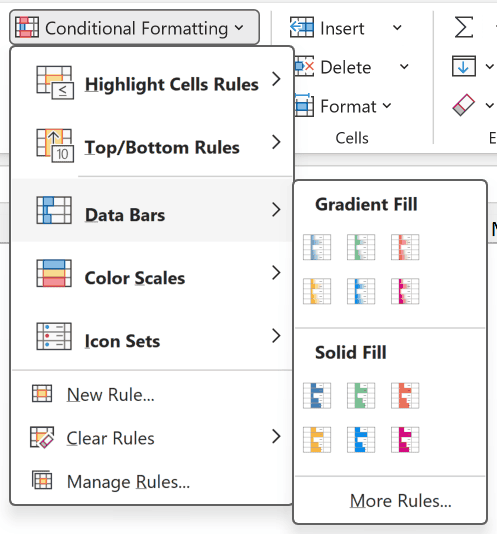
1. Select the cell with the percentage formula (D2), click the Home tab, then Conditional Formatting, then Data Bars, and choose a solid fill color.

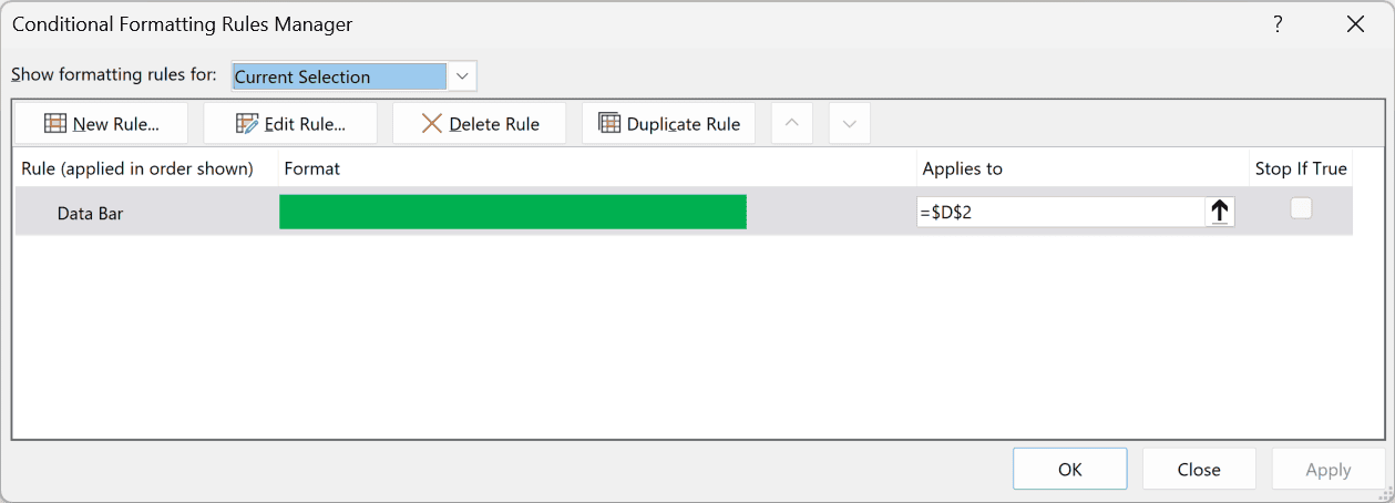
2. With D2 still selected, go back to Conditional Formatting, click Manage Rules, double-click the data bar rule, and set the Minimum to Number 0 and the Maximum to Number 1. This makes the bar scale from 0% to 100%.

Now every time you check off a task, the bar grows. Check all the boxes, and it fills the entire cell.

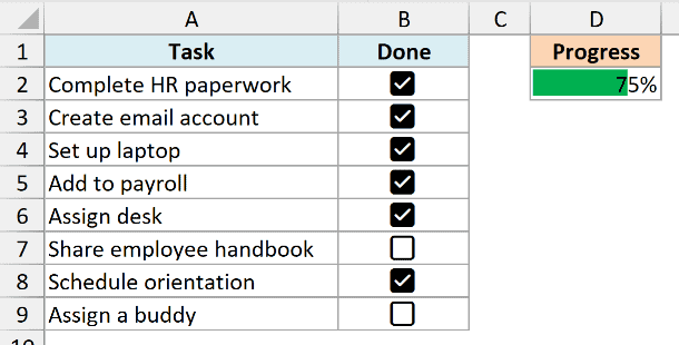
Pro Tip: Widen the cell with the progress bar (or merge a couple of cells) to make the bar look more like a proper progress bar in your dashboard.

How to Disable Checkboxes (Make Them Read-Only)

In some cases, you may want a checkbox that shows a status but can’t be clicked. For example, a summary checkbox that automatically gets checked when all the tasks in a list are done.

The trick is to apply the checkbox to a cell that has a formula returning TRUE or FALSE. When the underlying value comes from a formula, the checkbox becomes read-only, and clicking it does nothing.

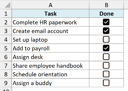
Below I have my onboarding task list, and in cell D5 I want a checkbox that gets checked automatically when all the tasks are complete.

Here is the formula I enter in cell D5:

=COUNTIF(B2:B9,TRUE)=COUNTA(A2:A9)

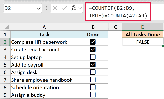
This returns TRUE only when the number of checked boxes equals the total number of tasks.

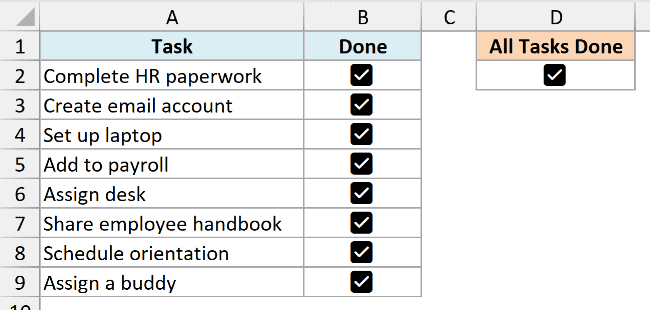
Now select cell D5 and insert a checkbox from the Insert tab (the same way as before). The checkbox shows the formula’s result, checks itself when all tasks are done, and can’t be toggled by clicking.

Checkboxes and Sheet Protection

If you protect a worksheet that has checkboxes, the checkboxes get locked too, and no one can check or uncheck them.

If you want people to be able to use the checkboxes on a protected sheet, unlock those cells before protecting the sheet. Select the cells with the checkboxes, press Ctrl + 1 to open the Format Cells dialog box, go to the Protection tab, and uncheck the Locked option.

Now when you protect the sheet (Review tab, then Protect Sheet), the rest of the sheet stays locked, but the checkboxes remain clickable.

I’ve covered locking and unlocking cells in detail in this article: How to Lock Cells in Excel

What About the Old Form Control and ActiveX Checkboxes?

Before these in-cell checkboxes were introduced, Excel had two other types of checkboxes, Form controls and ActiveX controls, both inserted from the Developer tab.

These older checkboxes are objects that float over the worksheet. They don’t sit inside a cell, they need to be linked to a cell manually to get a TRUE/FALSE value, and moving or aligning them is fiddly.

Now that the new checkboxes are here, I don’t recommend using the older ones. The only real advantage they still have is that, being objects, they can be placed anywhere on the worksheet, even on top of charts or images.

And if you’re on a version of Excel that doesn’t have the new checkboxes (such as Excel 2021 or Excel 2019), the Form control checkbox from the Developer tab is still your fallback option.

So this is everything you need to know about inserting and using checkboxes in Excel. Start with a simple checklist, and once you’re comfortable, try the interactive chart or the progress bar in your next tracker.

I hope you found this article helpful. If you have any questions or feedback, let me know in the comments section.

Other Excel Articles You May Also Like:

• How to Insert a Check Mark (Tick ✓) Symbol in Excel
• Excel To Do List Template (Free Download)
• Dynamic Excel Chart with Series Selection Check-box
• How to Insert a Scroll Bar in Excel
• How to Insert and Use a Radio Button (Option Button) in Excel