

If you want Excel to make a decision for you, returning one thing when a condition is true and something else when it is false, the IF function is what you need. It checks a condition you set and hands back the result you pick for each outcome.
In this article, I’ll show you how to use the IF function in Excel with practical examples, starting with a simple test and building up to nested conditions, combining IF with AND and OR, handling errors, and checking whether a cell contains specific text.
In Excel for Microsoft 365, Excel 2021, Excel 2024, and Excel for the web, you can also hand IF an entire range and the results spill into the cells below, so you get an answer for every row from a single formula.
Follow along with the example file
IF Function Examples.xlsx
IF Function Syntax
You may also see the IF function called an “IF statement” or an “if-then formula”. Here is the syntax of the IF function:
=IF(logical_test, value_if_true, [value_if_false])
- logical_test – the condition you want to check. This is anything that returns TRUE or FALSE, like
A2>100orB2="Yes". - value_if_true – what you want returned when the condition is TRUE. It can be text (in quotes), a number, or another formula.
- value_if_false – optional. What you want returned when the condition is FALSE. If you leave it out, IF returns FALSE when the condition isn’t met.
Pro Tip: Any text you want IF to return has to sit inside double quotes, like “Reorder”. Numbers and cell references don’t need quotes.
The IF function works in Excel for Microsoft 365, Excel 2024, 2021, 2019, 2016, and older versions, plus Excel on the web. So you can use it almost anywhere.
When to Use the IF Function
Use the IF function when you need to:
- Return one label or number when a condition is met, and a different one when it isn’t (like “Reorder” versus “OK”).
- Run a different calculation depending on whether a test passes (like applying a discount only above a certain quantity).
- Flag rows that meet a rule so you can filter, sort, or act on them.
Let me show you a few practical examples of how this works.
Example 1: A Simple IF Formula With a Text Result
Let’s start with the most common use, returning one of two text labels.
Below I have an inventory list with the product name in column A and the units in stock in column B. I want to flag which items are running low so someone knows to reorder them.
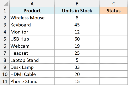
I want to mark any product with fewer than 20 units in stock as “Reorder”, and everything else as “OK”.
Here is the formula:
=IF(B2:B11<20,"Reorder","OK")
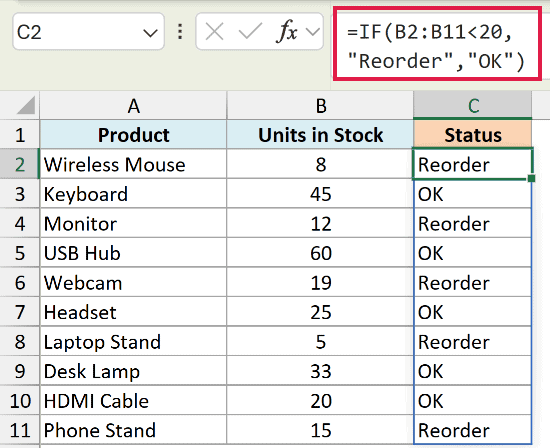
The first product has 8 units in stock, so the formula returns Reorder. Any product with 20 or more units returns OK.
Because I passed the whole range B2:B11 in one go, the formula spills a result down the column automatically. You type it once and Excel fills the rest.
Pro Tip: The spilling version works in Microsoft 365, Excel 2021, Excel 2024, and Excel for the web. On Excel 2019 or earlier, put =IF(B2<20,”Reorder”,”OK”) in the first cell and copy it down.
Example 2: Return a Calculated Value With IF
The result of an IF doesn’t have to be text. It can be a number or a whole calculation, and that’s where IF gets really useful.
Below I have an order list with the product in column A, the quantity ordered in column B, and the unit price in column C. I want to give a 10% discount on the unit price, but only for bulk orders.
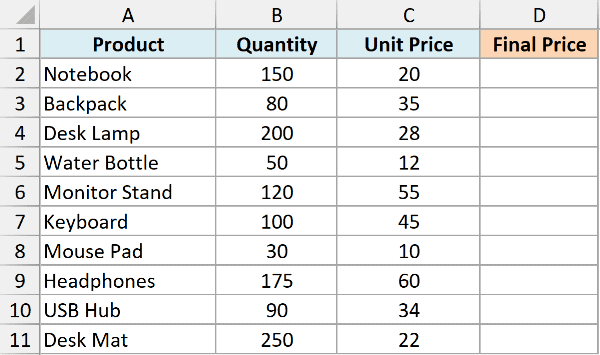
I want the discounted unit price when someone orders 100 units or more, and the regular price otherwise.
Here is the formula:
=IF(B2:B11>=100,C2:C11*0.9,C2:C11)
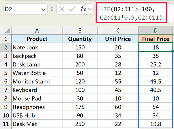
The first order is for 150 units at a $20 unit price. Since 150 is at least 100, the condition is TRUE, so the formula returns 18 (that’s 20 with 10% taken off).
Here the >= operator checks for “greater than or equal to” 100. When the test passes, C2:C11*0.9 does the math and returns the lower price. When it fails, the formula just returns the full price from column C.
Example 3: Nested IF for Multiple Conditions
An IF only handles two outcomes, TRUE or FALSE. When you have more than two, you put another IF inside the value_if_false slot. This is called a nested IF.
Below I have a task list with the task name in column A and the number of days until it’s due in column B. A negative number means the task is already past due. I want a status for each one.
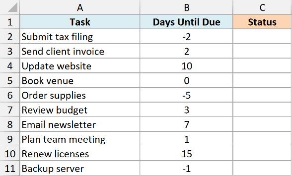
I want to show “Overdue” when the days are below 0, “Due Soon” when they’re 3 or fewer, and “On Track” for everything else.
Here is the formula:
=IF(B2:B11<0,"Overdue",IF(B2:B11<=3,"Due Soon","On Track"))
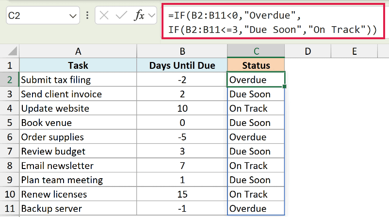
Here is how this reads for a single task:
- The first IF checks if the days are below 0. A task at -2 days returns Overdue.
- If that’s FALSE, the second IF takes over and checks if the days are 3 or fewer. A task at 2 days returns Due Soon.
- If both are FALSE, the last value kicks in. A task at 10 days returns On Track.
Each IF only runs when the one before it comes back FALSE, so the order of your tests matters.
Pro Tip: Once you’re stacking three or more conditions, the IFS function is easier to read. You list each condition and result as a pair, with no closing brackets to count.
Example 4: Using IF With the AND Function
Sometimes a row only counts when two things are true at the same time. That’s the job of the AND function, which you drop straight into the logical_test.
Below I have an order list with the order ID in column A, the order amount in column B, and whether it’s from a new customer in column C. I want to catch orders that need a manual review.
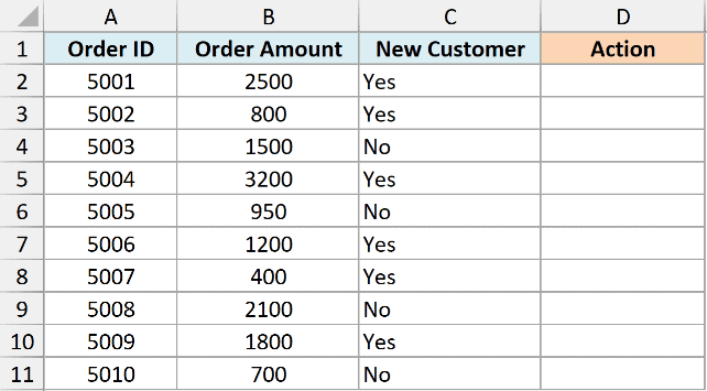
I want to flag an order for “Review” only when the amount is over 1000 and it’s from a new customer, otherwise “Auto-Approve”.
Here is the formula:
=IF(AND(B2>1000,C2="Yes"),"Review","Auto-Approve")
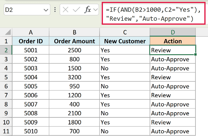
The first order is for 2500 from a new customer. Both conditions are TRUE, so AND returns TRUE and the formula returns Review. If either one had been false, it would return Auto-Approve.
AND collapses its conditions into a single TRUE or FALSE, so it doesn’t spill across a range on its own. Here I keep the formula per-row and copy it down. In 365 you could spill an equivalent using =IF((B2:B11>1000)*(C2:C11="Yes"),"Review","Auto-Approve").
Example 5: Using IF With the OR Function
The OR function is the flip side of AND. It returns TRUE when at least one of your conditions is met, so it’s the right pick when any single reason is enough.
Below I have a product list with the product in column A, the units in stock in column B, and the days until it expires in column C. I want to spot items worth putting on a promotion.
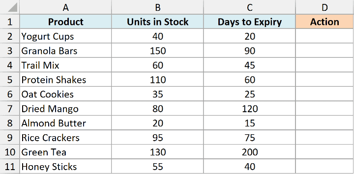
I want to mark a product “Promote” if it’s overstocked (more than 100 units) or close to expiring (fewer than 30 days), and “Keep” otherwise.
Here is the formula:
=IF(OR(B2>100,C2<30),"Promote","Keep")
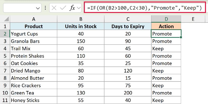
The first product has 40 units in stock but only 20 days until it expires. The stock condition is FALSE, but the expiry condition is TRUE, and since OR only needs one to be true, the formula returns Promote.
A row returns Keep only when both conditions are FALSE, meaning the item is neither overstocked nor expiring soon.
Also check: How to Use IF Function with OR in Excel
Example 6: Handle Errors With IF to Avoid #DIV/0!
IF is handy for stopping errors before they happen. A classic case is dividing by a cell that might be zero, which throws a #DIV/0! error.
Below I have a campaign report with the campaign in column A, the conversions in column B, and the clicks in column C. I want a conversion rate, but some campaigns have zero clicks.
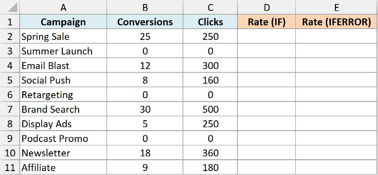
I want to divide conversions by clicks, but return 0 whenever the clicks are 0, so I never see a #DIV/0! error.
Here is the formula:
=IF(C2:C11=0,0,B2:B11/C2:C11)
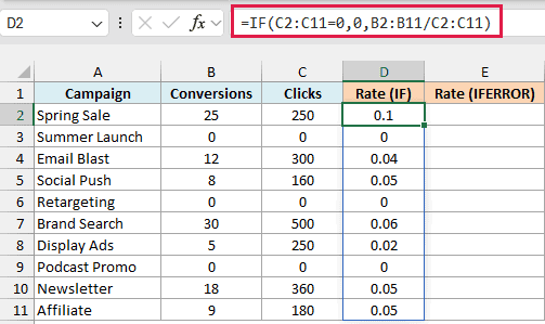
The IF checks the clicks first. When the clicks are 0, it returns 0 and never attempts the division. When the clicks are anything else, like 250 clicks with 25 conversions, it returns the rate of 0.1.
This works because you’re checking the exact thing that would cause the error. If you instead want to catch any error type, not just a zero, the IFERROR function is shorter.
Here is the same result with IFERROR:
=IFERROR(B2:B11/C2:C11,0)
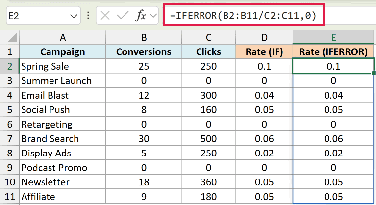
IFERROR runs the division, and if the result is any error at all, it returns 0 instead. It’s cleaner here, but IF gives you more control when you want to test one specific condition.
Example 7: Check if a Cell Contains Specific Text
A common question is how to make IF react to text that appears anywhere inside a cell, not just an exact match. You do that by pairing IF with SEARCH and ISNUMBER.
Below I have an order list with the item description in column A. Some descriptions mention a gift, and I want to flag those so they get special packaging.
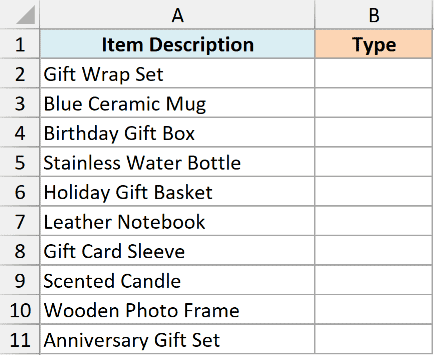
I want to return “Gift” when the description contains the word gift anywhere in it, and “Regular” when it doesn’t.
Here is the formula:
=IF(ISNUMBER(SEARCH("gift",A2:A11)),"Gift","Regular")
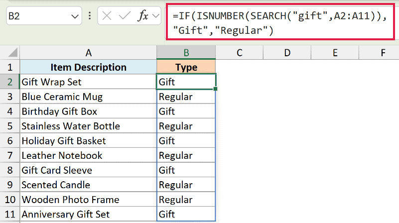
A description like “Gift Wrap Set” returns Gift, while “Blue Ceramic Mug” returns Regular. Here is what each piece is doing:
- SEARCH(“gift”,A2) looks for the word gift inside the cell and returns its position number if it finds it, or a #VALUE! error if it doesn’t.
- ISNUMBER turns that into TRUE or FALSE. A position number is TRUE, an error is FALSE.
- IF then returns Gift or Regular based on that TRUE/FALSE.
Pro Tip: SEARCH ignores case, so “gift”, “Gift”, and “GIFT” all match. There are more ways to check if a cell contains partial text in Excel if you need case-sensitive matching or a full list of matches.
Tips & Common Mistakes
A few things that trip people up with the IF function:
- Put text you type directly into the formula in double quotes. Use “Reorder”, for example. Without quotes, Excel reads it as a name and may return #NAME?. Numbers, cell references, and formulas do not need quotes.
- The logical_test just needs to return TRUE or FALSE. Anything that evaluates to a TRUE/FALSE works, whether it’s a comparison like
A2>100, a text check likeB2="Yes", or a function like AND, OR, or ISNUMBER. - Leaving out value_if_false returns FALSE, not a blank. If you do not want anything shown when the test fails, use “” (an empty pair of quotes) as the last argument. The result looks blank but contains an empty string.
- Watch the order in a nested IF. Excel checks the conditions top to bottom and stops at the first TRUE, so list your tightest condition first or a later one may never get reached.
- Dates work just like numbers in IF. Excel stores dates as numbers, so you can compare them with
>,<, and>=. For a range check, see how to check if a date is between two dates. - Don’t nest more than you have to. Long nested IFs are hard to read and edit. For many tiers, reach for the IFS function, and for looking up a value in a table, a lookup function is cleaner than a stack of IFs.
Wrapping Up
The IF function is one of the first functions worth getting comfortable with, since so much of what you do in Excel comes down to “if this, then that.” Start with a single condition, then layer in nested IFs, AND, OR, and error handling as your rules get more involved.
I hope you found this tutorial helpful. If you get stuck on an IF formula, it usually comes down to a missing set of quotes or the order of your conditions.
Other Excel Articles You May Also Like:
