Check IF a Date is Between Two Given Dates in Excel (Easy Formulas)

A common thing many Excel users need to check when working with dates is whether a date is between two given dates.

A simple use case of this could be when you need to check whether the date of submission of a report was within the given dates or not. Based on this, you can highlight what reports were submitted after the deadline.

Excel doesn’t have a BETWEEN function, but you don’t need one. You just check two things: the date is on or after the start date, and it’s on or before the end date.

In this tutorial, I will show you how to check if the date is between two given dates or not.

I’ll also cover how to return a value based on which date range a date falls in, and a couple of issues that can give you unexpected results.

Check If a Date Is Between Two Dates Using IF + AND

While many Excel users are quite comfortable using the IF formula, when you have multiple conditions to check, I prefer using the combination of IF and AND formula instead.

The AND formula lets you check multiple conditions at once. In the spilling formula below, I do the same job by multiplying the two checks, and I’ll explain why right after the formula.

Below I have a data set of store coupons with the dates each coupon is valid from and to, and the date it was used, and I want to check whether each coupon was used within its valid dates in column E.

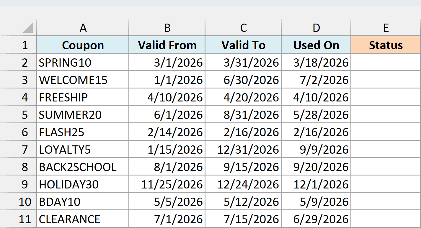
Here is the formula that will do this:

=IF((D2:D11>=B2:B11)*(D2:D11<=C2:C11),"Valid","Not Valid")

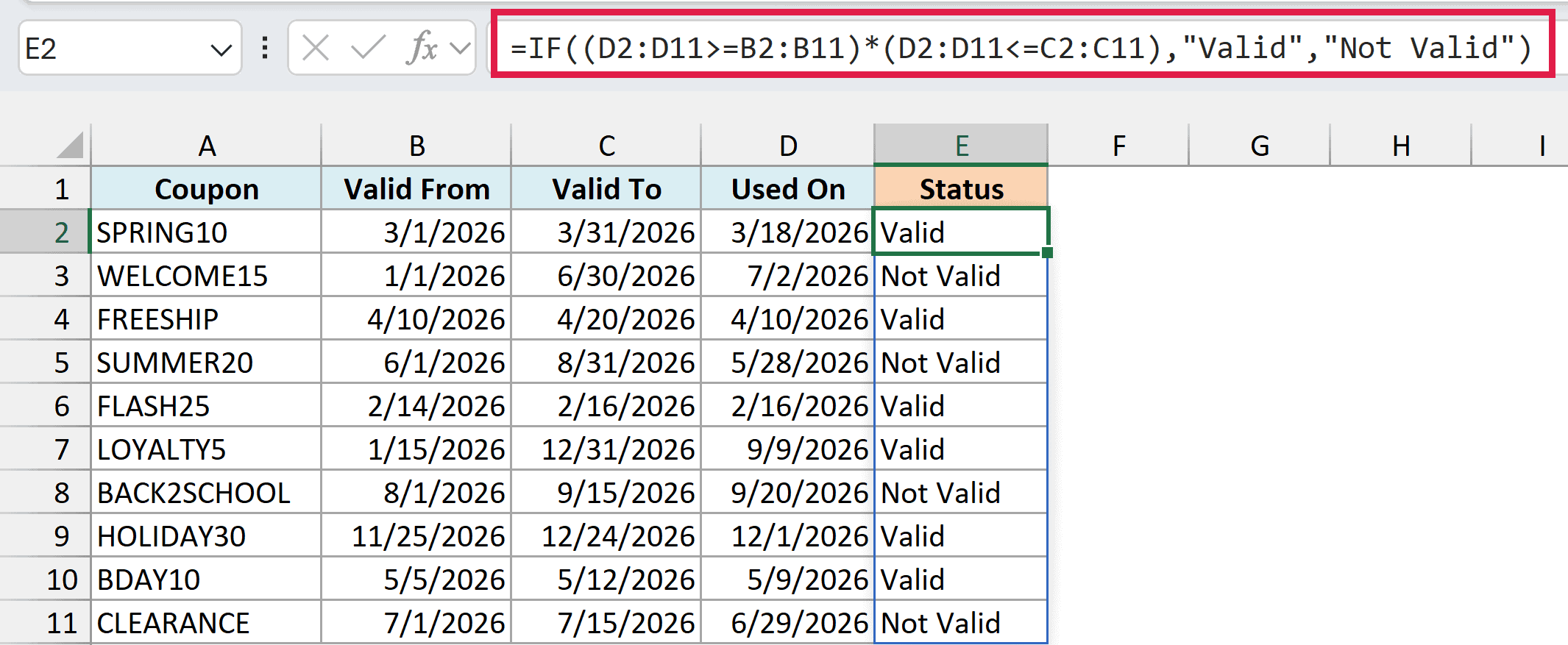
You only need to enter this formula in cell E2, and it spills down to E11 on its own.

It returns ‘Valid’ when the coupon was used between its two dates, and ‘Not Valid’ when it was used before the start date or after the end date.

How this formula works:

• (D2:D11>=B2:B11) – This checks whether each Used On date is on or after the Valid From date in the same row. It gives a list of 10 TRUE or FALSE values.
• (D2:D11<=C2:C11) – This checks whether each Used On date is on or before the Valid To date, again giving 10 TRUE or FALSE values.
• Multiplying the two – In the back end, Excel considers TRUE as 1 and FALSE as 0. So a row gets 1 only when both checks are TRUE, and 0 when either one is FALSE, which is exactly what the AND function does.
• IF(…,”Valid”,”Not Valid”) – The IF function returns ‘Valid’ for every 1 and ‘Not Valid’ for every 0.

You may wonder why there’s no AND function in this formula. That’s because the AND function looks at everything you give it and returns one single TRUE or FALSE, so AND(D2:D11>=B2:B11,D2:D11<=C2:C11) would give you one answer for all 10 coupons instead of one per row.

Also note that the formula uses >= and <=, so a coupon used on its start date or its end date counts as valid.

You can see this with FREESHIP (used on 4/10/2026, its first valid day) and FLASH25 (used on 2/16/2026, its last valid day).

If you don’t want to include the start and end dates, use > and < instead of >= and <=.

The spilling formulas in this article work in Excel 365 and Excel 2021 or later. If you’re on Excel 2019 or earlier, use the copy-down version shown with each method.

If you’re using Excel 2019 or earlier (or you simply prefer the AND function), enter the below formula in cell F2 and then copy it down the range:

=IF(AND(D2>=B2,D2<=C2),"Valid","Not Valid")

This gives the same result in column F of the example file.

Note that I have still used an IF function in the above formula, however, I didn’t have the need to use two IF functions (like in the nested IF method later in this article).

Since I had to check for both the conditions, I did that using the AND function instead.

The AND function would return TRUE if both the conditions are true, and it would return FALSE if any or both the conditions are false.

And since I needed a more descriptive output instead of a simple TRUE or FALSE, I have used an IF function where it would give me ‘Valid’ in case the result is TRUE and ‘Not Valid’ in case the result is FALSE.

Also read: Count Between Two Numbers in Excel (COUNTIF / COUNTIFS)

Dates Need to Be in the Right Format (Text Dates)

In all the formulas, the underlying principle is to compare the value of the given date with the start and the end date.

If the value of the given date is in between the start and the end date, then it occurs in between these two dates, else it does not.

However, in some cases, you may see some unexpected results. Here’s the first common pitfall you need to be aware of when comparing dates in Excel.

Dates and time values are stored as numbers in the back-end in Excel. So when you compare two dates, you’re essentially comparing two numbers.

You may think that the date looks nothing like a number (for example 01 January 2023), but remember that dates are formatted to show up differently in the cell in Excel, while in the back-end these are still numbers.

For example, a cell may show 01 January 2023, but in the backend, the value of this cell would be 44927. That’s because Excel counts days starting from 01 January 1900, which is day 1.

Now, if your dates are in the right format, all is well.

But there is also a possibility that your date is in a format that Excel does not recognize as a date, which means that instead of a number in the back end, it ends up being considered a text string.

For example, with US date settings, 04.15.2026 (with dots) is not a valid date format in Excel.

So if you have this in a cell in Excel, it would be considered a text string, and using this to compare it with other dates can give you incorrect results.

Below I have the coupon data again, where two of the Used On dates were entered with dots, and I want to see what the formula returns for them in column E.

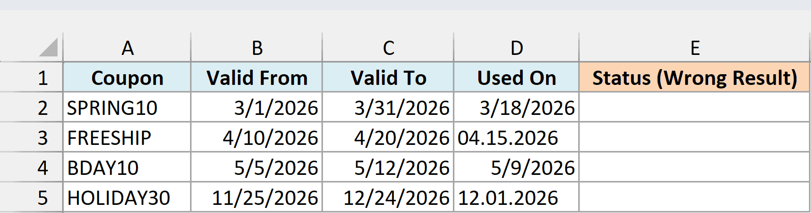
Here is the same formula we used earlier:

=IF((D2:D5>=B2:B5)*(D2:D5<=C2:C5),"Valid","Not Valid")

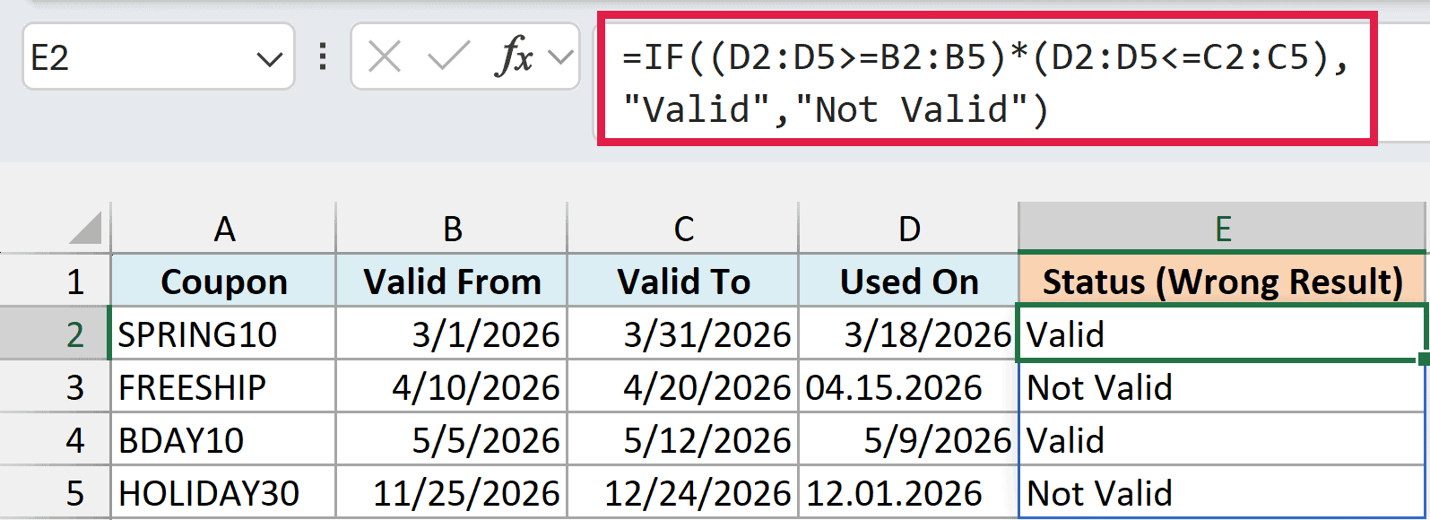
FREESHIP (04.15.2026) and HOLIDAY30 (12.01.2026) show ‘Not Valid’, even though both dates are clearly inside their valid range. Excel treats any text as larger than any number in a comparison, so the text passes the start-date check but fails the end-date check.

Notice that there’s no error to warn you. You just get a wrong answer, which is why this one is easy to miss.

A quick way to spot these cells is to check which values are real numbers. Enter the below formula in cell F2:

=ISNUMBER(D2:D5)

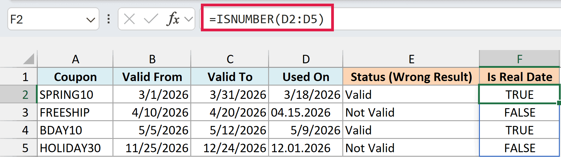
The ISNUMBER function returns FALSE for the two text dates and TRUE for the real ones. You can also spot them visually, as text sits on the left of the cell by default while real dates line up on the right.

If you’re using Excel 2019 or earlier, enter the below formula in cell F2 and then copy it down the range:

=ISNUMBER(D2)

Once you know which cells are text, you can convert the text to dates, and the formula will give you the right result.

Bottom line – When comparing dates in Excel, make sure that the dates are in the right format

Also read: How to Change Date Format In Excel?

Dates May Have a Time Part That’s Hidden

Here’s the second pitfall. Just like dates, time values are also stored as numbers in the backend in Excel.

While a whole number would indicate a full day, the decimal part would indicate the portion of the day or the time value for that day.

For example, if you have 01-01-2023 18:00:00 in a cell in Excel, in the backend it would be 44927.75, where 44927 means 01-01-2023 and 0.75 means 18:00:00.

Now, here’s the problem that you can encounter when checking whether a date lies in between two given dates. You may clearly see that the date is in between the two given dates, but Excel may give you a different result.

This can happen because most of the time when people work with dates and times, the time portion is hidden so that you only see the date but you do not see the time value.

Below I have some coupons where the Used On dates in column D also have a time part, but the cells only show the date, and I want to check whether each coupon was used within its valid dates in column F.

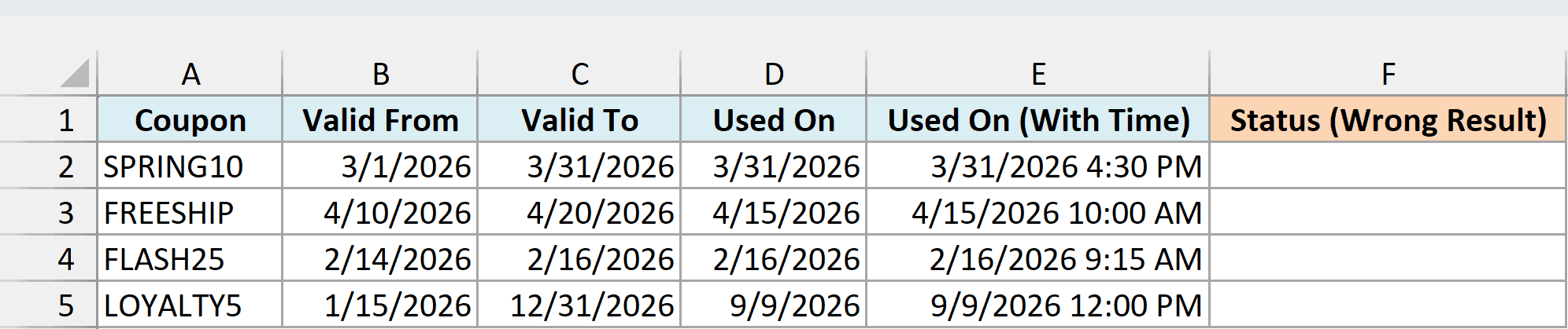
Here is the formula we used earlier:

=IF((D2:D5>=B2:B5)*(D2:D5<=C2:C5),"Valid","Not Valid")

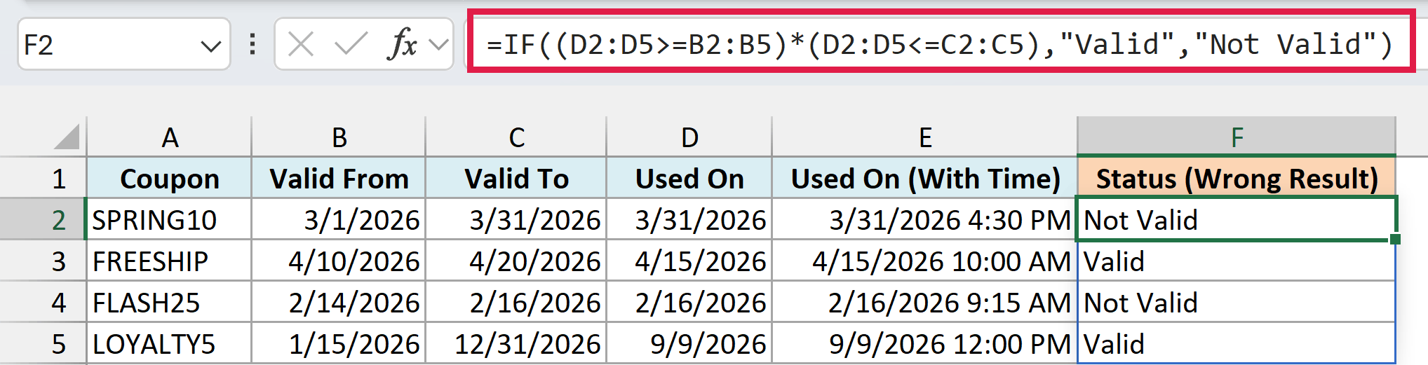
SPRING10 shows ‘Not Valid’, even though it was used on 3/31/2026 and the coupon is valid till 3/31/2026. The same thing happens with FLASH25.

While you can clearly see that these dates look exactly the same, what you do not see is that there is a time value in the cell that is hidden.

Column E of the example file shows the same values with the time visible, and SPRING10 was used at 4:30 PM on 3/31/2026.

When Excel compares 3/31/2026 4:30 PM with 3/31/2026 (which is midnight), it considers the first one larger, so the <= check fails (which it rightly should).

While this is not such a common scenario, if this happens, it can sometimes stump even advanced Excel users.

To fix this, you can use the INT function to drop the time part before comparing. Enter the below formula in cell G2:

=IF((INT(D2:D5)>=B2:B5)*(INT(D2:D5)<=C2:C5),"Valid","Not Valid")

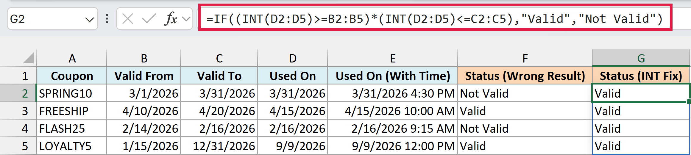
The INT function removes the decimal part of a number, so INT(D2:D5) keeps only the date. Now SPRING10 and FLASH25 both show ‘Valid’.

If you’re using Excel 2019 or earlier, enter the below formula in cell G2 and then copy it down the range:

=IF(AND(INT(D2)>=B2,INT(D2)<=C2),"Valid","Not Valid")

If you don’t need the time at all, you can also remove the time from the dates in the cells themselves, and the original formula will work as is.

Check If a Date Is Within a Date Range Given in Cells

So far, every coupon had its own start and end date. But quite often, you have one date range for the whole list, such as a sale period, and you want to check every date against it.

Below I have a list of orders with their order dates, and the sale start and end dates in cells F1 and F2, and I want to check whether each order was placed during the sale in column C.

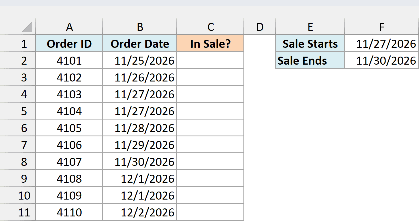
Here is the formula that will do this:

=IF((B2:B11>=F1)*(B2:B11<=F2),"Yes","No")

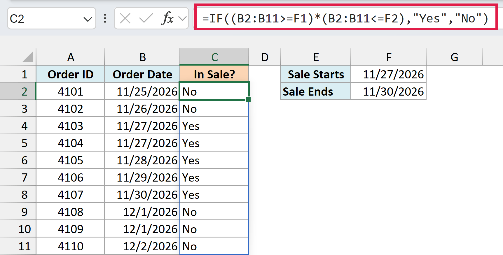
The formula compares every order date in B2:B11 with the same start date in F1 and the same end date in F2. Orders placed from 11/27/2026 to 11/30/2026 get ‘Yes’, and the rest get ‘No’.

Keeping the dates in cells (instead of typing them inside the formula) is useful because you can change the sale dates anytime, and the results update automatically.

If you’re using Excel 2019 or earlier, enter the below formula in cell C2 and then copy it down the range:

=IF(AND(B2>=$F$1,B2<=$F$2),"Yes","No")

The dollar signs lock F1 and F2, so every row keeps comparing with the same sale dates when you copy the formula down.

Using Nested IF Formula

Another easy way to check whether a date is in between two given dates is by using a simple IF formula.

And since we need to check for two conditions, we would need to use two IF formulas. And when you use an IF formula within another IF formula, that is called the nested IF construct.

Below I have the same coupon data set with the valid from and valid to dates and the date each coupon was used, and I want to check whether each coupon was used within its valid dates in column E.

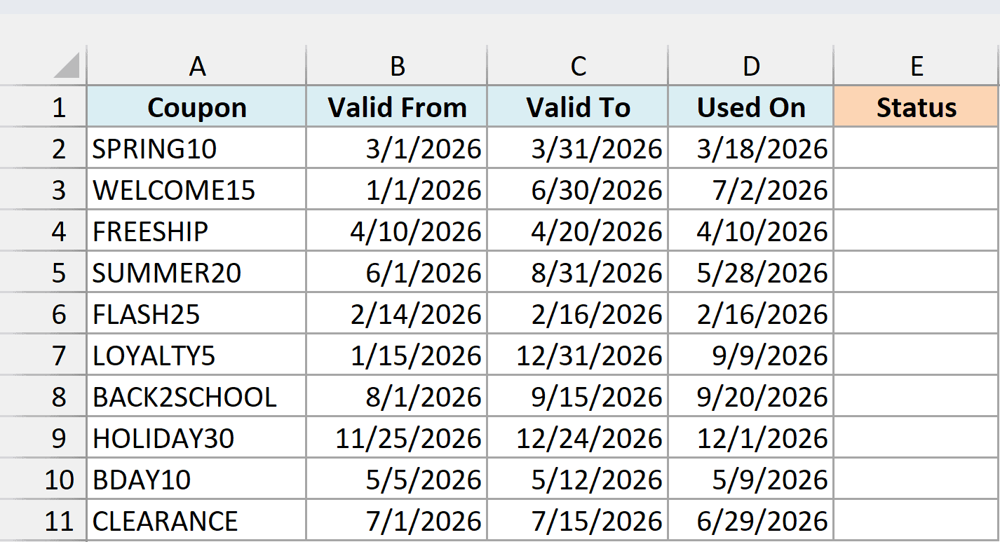
This can easily be done using the below nested IF formula:

=IF(D2:D11>=B2:B11,IF(D2:D11<=C2:C11,"Valid","Not Valid"),"Not Valid")

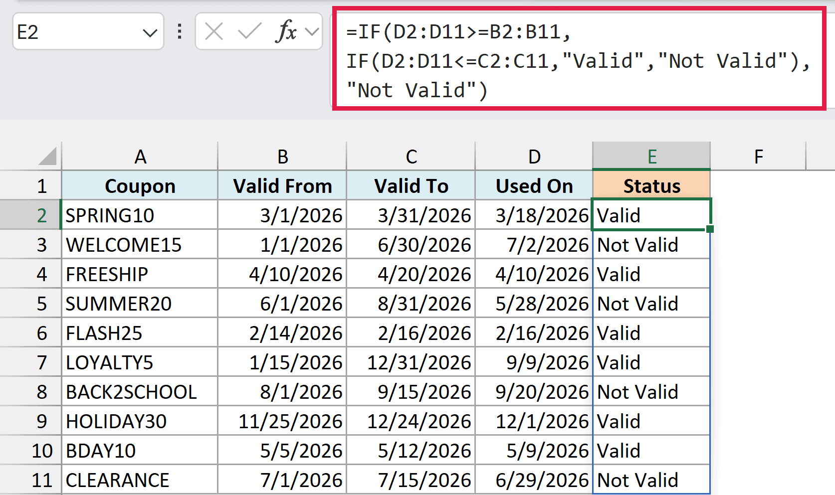
The above formula would return ‘Valid’ if the date lies in between the two given dates, and it would return ‘Not Valid’ in case the date is either before the coupon’s start date or after its end date.

Now let me quickly explain how this formula works.

I first used an IF formula to check whether the date is on or after the valid from date or not.

Based on this condition, I need to specify what the formula should do in case this condition is true, and what it should do in case the condition is not true.

But since I have two conditions to check, immediately after I checked the first condition, I use the second IF function to check for the other condition (which is whether the date is on or before the valid to date or not).

Since the IF function takes 3 arguments (the condition, value when the condition is True, and value when the condition is False), for the second IF function, I specify ‘Valid’ as the second argument, as it has satisfied both the conditions.

And I specify ‘Not Valid’ as the third argument, because it satisfies the first IF condition, but it fails the second IF condition.

And then finally, I specify ‘Not Valid’ as the third argument for the first IF function. This is what you get when the condition in the first IF function fails, so the formula never goes to the second IF function.

Since I had only two conditions to check, I have used two IF functions where the second function is nested within the first one.

Pro Tip: In case you have more than two conditions to check, you can further nest these IF functions (although it tends to get a bit complicated after a few).

If you’re using Excel 2019 or earlier, enter the below formula in cell E2 and then copy it down the range:

=IF(D2>=B2,IF(D2<=C2,"Valid","Not Valid"),"Not Valid")

Also read: Avoid Nested IF Function in Excel…VLOOKUP to Rescue

If a Date Is Between Two Dates, Return a Value (Multiple Date Ranges)

Sometimes you don’t just want to know whether a date falls within a range. You have a few date ranges, each with its own name, and you want to get the name of the range the date falls in.

Below I have a list of school events with their dates, and a table of school terms with their start and end dates on the right, and I want to get the term for each event in column C.

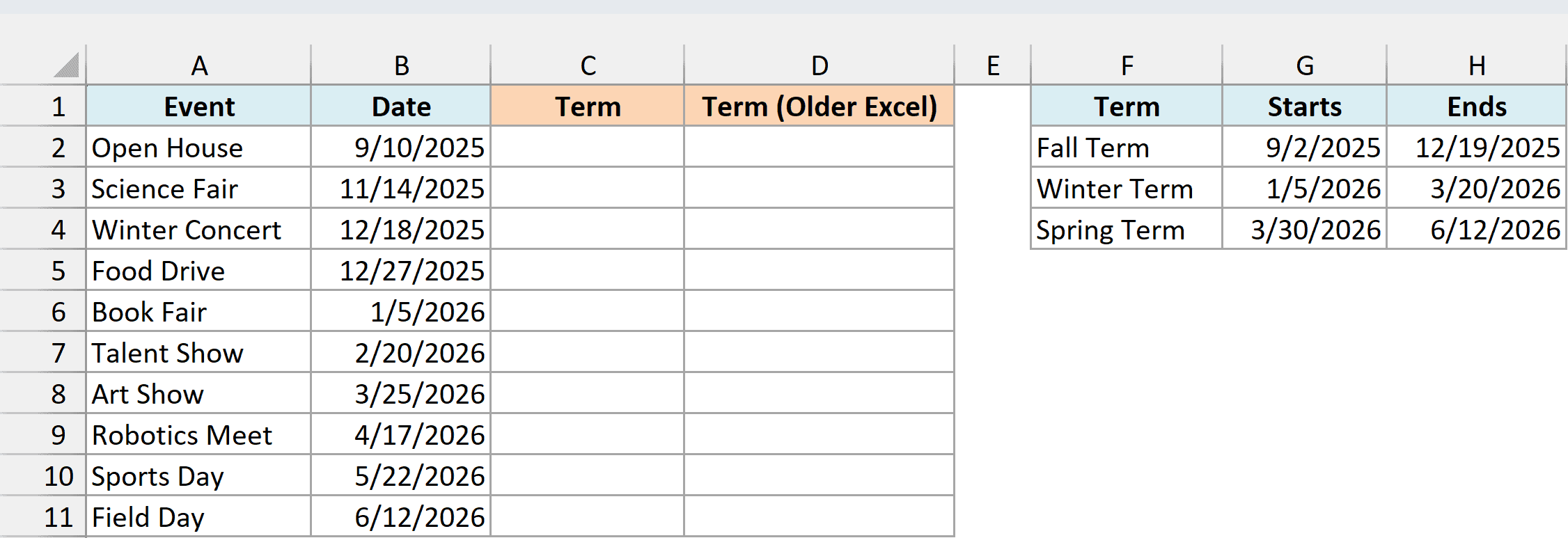
Here is the formula that will do this:

=XLOOKUP(1,(B2>=$G$2:$G$4)*(B2<=$H$2:$H$4),$F$2:$F$4,"School Break")

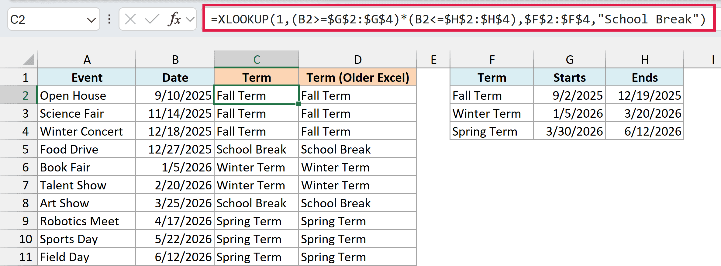
Enter this formula in cell C2 and copy it down to C11. Food Drive (12/27/2025) and Art Show (3/25/2026) get ‘School Break’, as they fall in the gaps between terms.

How this formula works:

• (B2>=$G$2:$G$4)*(B2<=$H$2:$H$4) – This checks the event date against all three terms at once. Just like in the first method, multiplying the two checks gives 1 for the term where the date is on or after the start and on or before the end, and 0 for the others.
• XLOOKUP(1,…,$F$2:$F$4,…) – The XLOOKUP function looks for that 1 and returns the term name from the same position in F2:F4.
• “School Break” – This is what the XLOOKUP function returns when there’s no 1 at all, which means the date doesn’t fall in any term.

The dollar signs keep the term table fixed when you copy the formula down. If your date ranges overlap, the XLOOKUP function returns the first matching range from the top.

The XLOOKUP function is available in Excel 365 and Excel 2021 or later. If you’re using Excel 2019 or earlier, enter the below formula in cell C2 and then copy it down the range:

=IFERROR(LOOKUP(2,1/((B2>=$G$2:$G$4)*(B2<=$H$2:$H$4)),$F$2:$F$4),"School Break")

This version is in column D of the example file, and it gives the same result here. Dividing 1 by the 1s and 0s turns the non-matching terms into #DIV/0! errors.

Since 2 is bigger than any 1 in that list, the LOOKUP function skips the errors and lands on the last 1, which is the matching term. When nothing matches, the LOOKUP function returns an error, and the IFERROR function turns it into ‘School Break’.

One difference to keep in mind: if your date ranges overlap, this version returns the last matching range, while the XLOOKUP version returns the first.

Check If the Date Occurs on Weekend

A common use case when working with dates in project management is to identify whether a date occurs on a weekend or not.

If you’re checking this manually, you would check whether a date is a Saturday or Sunday. But when working with dates in Excel, you can use the WEEKDAY function that can easily do this for you.

Below I have a data set where I have some delivery dates in column A, and I want to check whether these dates occur on a weekend or not in column B.

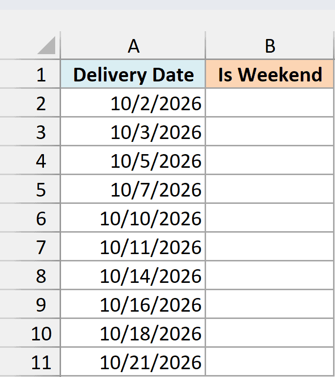
For the purpose of this tutorial, I would consider Saturday and Sunday as the weekend days.

Below is the formula that will do this for you:

=WEEKDAY(A2:A11,2)>5

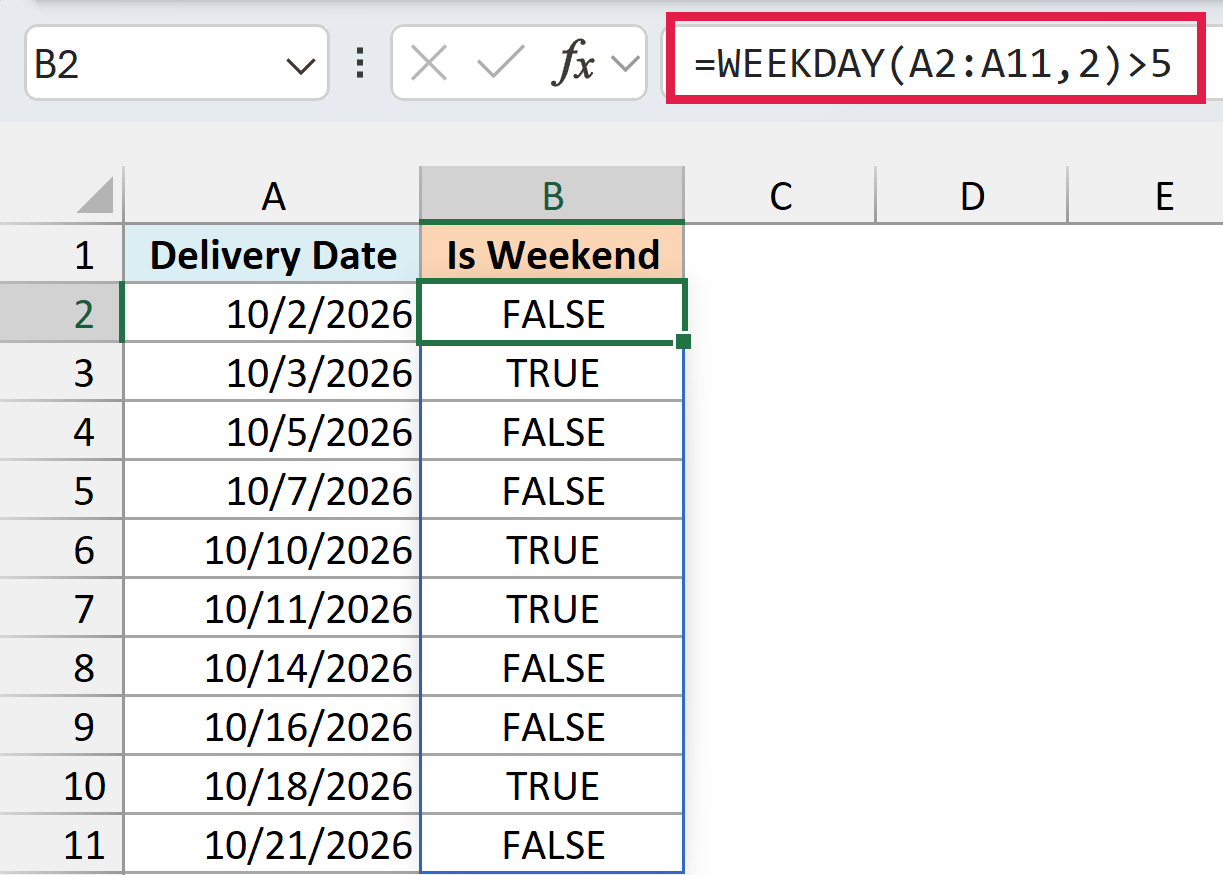
If the date occurs on a Saturday or Sunday, it will give you a TRUE, else it will give a FALSE.

The above WEEKDAY formula checks the serial number of the date, and returns a number that corresponds to the weekday number for that date.

With 2 as the second argument, if it’s a Monday, it would return 1, if it’s a Tuesday it would return 2, and so on till Sunday, which returns 7.

Since the condition that I’m checking is whether the weekday result is more than 5, it would return TRUE if the date is on a weekend, and it would return FALSE if it’s on a weekday.

If you want the result to be more meaningful, you can use the below IF formula, which will return ‘Weekday’ in case the date occurs on a weekday and ‘Weekend’ in case the date occurs on a weekend.

=IF(WEEKDAY(A2:A11,2)>5,"Weekend","Weekday")

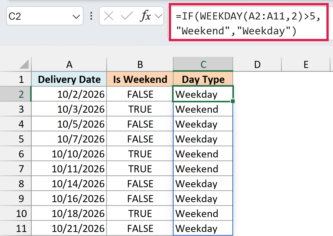
If you’re using Excel 2019 or earlier, enter the below formula in cell B2 and then copy it down the range:

=WEEKDAY(A2,2)>5

And for the Weekday and Weekend labels, enter the below formula in cell C2 and copy it down:

=IF(WEEKDAY(A2,2)>5,"Weekend","Weekday")

If you want to color the weekend dates instead of labeling them, you can highlight weekend dates with conditional formatting.

Also read: Calculating Time In Excel

In this tutorial, I showed you a couple of simple formulas that you can use to check whether a date is between two given dates or not.

I’ve also mentioned some of the pitfalls you should be aware of when comparing dates in Excel.

I hope you found this Excel tutorial useful.

Other Excel Tutorials you may also like:

• Calculate the Number of Months Between Two Dates in Excel
• How to Calculate the Number of Days Between Two Dates in Excel
• How to Add or Subtract Days to a Date in Excel
• How to Stop Excel from Changing Numbers to Dates Automatically
• How to Add Months to Date in Excel
• How to Get the Number of Days in a Month in Excel?
• Get Day Name from Date in Excel
• How to SUM Values Between Two Dates (using SUMIFS formula)
• How to Use Multiple Criteria in Excel COUNTIF and COUNTIFS Function