

Excel XLOOKUP function has finally arrived.
If you have been using VLOOKUP or INDEX/MATCH, I am sure you’ll love the flexibility that the XLOOKUP function provides.
In this tutorial, I will cover everything there is to know about the XLOOKUP function and some examples that will help you know how to best use it.
So let’s get started!
Follow along with the example file
XLOOKUP Function Examples.xlsx
What is XLOOKUP?
XLOOKUP is a lookup function available in Microsoft 365, Excel 2021, Excel 2024, and Excel for the web. It is a new and improved version of the VLOOKUP/HLOOKUP function.
It does everything VLOOKUP used to do, and much more.
XLOOKUP is a function that allows you to quickly look for a value in a dataset (vertical or horizontal) and return the corresponding value in some other row/column.
For example, if you’ve got the scores for students in an exam, you can use XLOOKUP to quickly check how much a student has scored using the name of the student.
The power of this function will become even more clear as I deep dive into some XLOOKUP examples later in this tutorial.
When to Use XLOOKUP
XLOOKUP replaces VLOOKUP, HLOOKUP, and most INDEX/MATCH formulas. Reach for it when you want to:
- Look up a value and return a match from any column, including one to the left of the lookup column (something VLOOKUP can’t do).
- Return your own message when a value isn’t found, without wrapping the formula in IFERROR.
- Pull back an entire row or column in a single formula, with the result spilling automatically.
- Get an exact match by default, so an accidental approximate match never gives you the wrong result.
- Search from the bottom up to grab the last matching record.
- Handle both vertical and horizontal lookups with the same function.
XLOOKUP Function Syntax
Below is the syntax of the XLOOKUP function:
=XLOOKUP(lookup_value, lookup_array, return_array, [if_not_found], [match_mode], [search_mode])

If you’ve used VLOOKUP, you’ll notice that the syntax is quite similar, with some awesome additional features of course.
Don’t worry if the syntax and argument look a bit too much. I cover these with some easy XLOOKUP examples later in this tutorial that will make it crystal clear.
XLOOKUP function can take 6 arguments (3 mandatory and 3 optional):
- lookup_value – the value that you’re looking for
- lookup_array – the array in which you’re looking for the lookup value
- return_array – the array from which you want to fetch and return the value (corresponding to the position where the lookup value is found)
- [if_not_found] – the value to return in case the lookup value is not found. In case you don’t specify this argument, a #N/A error would be returned
- [match_mode] – Here you can specify the type of match you want:
- 0 – Exact match, where the lookup_value should exactly match the value in the lookup_array. This is the default option.
- -1 – Looks for the exact match, but if it isn’t found, returns the next smaller item/value
- 1 – Looks for the exact match, but if it isn’t found, returns the next larger item/value
- 2 – To do partial matching using wildcards (* or ?), with ~ to escape a literal wildcard
- [search_mode] – Here you specify how the XLOOKUP function should search the lookup_array
- 1 – This is the default option where the function starts looking for the lookup_value from the top (first item) to the bottom (last item) in the lookup_array
- -1 – Does the search from bottom to top. Useful when you want to find the last matching value in the lookup_array
- 2 – Performs a binary search where the data needs to be sorted in ascending order. If not sorted, this can give error or wrong results
- -2 – Performs a binary search where the data needs to be sorted in descending order. If not sorted, this can give error or wrong results
The match_mode and search_mode arguments are optional, but they are what make XLOOKUP so flexible. Here is what each value does:
| match_mode | What it does |
|---|---|
| 0 (default) | Exact match. Returns #N/A if nothing matches. |
| -1 | Exact match, or the next smaller item if there is no exact match. |
| 1 | Exact match, or the next larger item if there is no exact match. |
| 2 | Wildcard match (use * and ? in the lookup value). |
| search_mode | What it does |
|---|---|
| 1 (default) | Search first to last (top to bottom). |
| -1 | Search last to first (bottom to top), handy for finding the last matching row. |
| 2 | Binary search on data sorted in ascending order. |
| -2 | Binary search on data sorted in descending order. |
XLOOKUP Function Examples
Now let’s look at some practical XLOOKUP examples.
These examples will help you better understand how XLOOKUP works, how it’s different from VLOOKUP and INDEX/MATCH and some enhancements and limitations of this function.
Example 1: Fetch a Lookup Value
Suppose you have the following dataset and you want to fetch the math score for Greg (the lookup value).

Below is the formula that does this:
=XLOOKUP(F2,A2:A15,B2:B15)

In the above formula, I have just used the mandatory arguments where it looks for the name (from top to bottom), finds an exact match, and returns the corresponding value from B2:B15.
One obvious difference between the XLOOKUP and VLOOKUP functions is the way they handle lookup array. In VLOOKUP, you have the entire array where the lookup value is in the left-most column and then you specify the column number from where you want to fetch the result. XLOOKUP, on the other hand, allows you to choose lookup_array and return_array separately
One instant benefit of having the lookup_array and return_array as separate arguments means that now you can look to the left. VLOOKUP had this limitation where you can only look up and find a value that is to the right. But with XLOOKUP, that limitation is gone.
Here is an example. I have the same dataset, where the name is on the right and the return_array is on the left.

Below is the formula that I can use to get the score for Greg in Math (which means looking to the left of the lookup_value)
=XLOOKUP(F2,D2:D15,A2:A15)

XLOOKUP solves another major issue – In case you insert a new column, or move columns around, the resulting data would still be correct. VLOOKUP would likely break or give an incorrect result in such cases as most times the column index value is hard-coded.
Example 2: Lookup and Fetch an Entire Record
Let’s take the same data as an example.
In this case, I don’t want to just fetch Greg’s score in Math. I want to get the scores in all the subjects.

In this case, I can use the below formula:
=XLOOKUP(F2,A2:A15,B2:D15)

The above formula uses a return_array range that is more than a column (B2:D15). So when the lookup value is found in A2:A15, the formula returns the entire row from the return_array.
Also, you can not delete just cells that are part of the array that were automatically populated. In this example, you can not delete H2 or I2. If you try, nothing would happen. If you select these cells, the formula in the formula bar would be grayed out (indicating that it can not be changed)
You can delete the formula in cell G2 (where we originally entered it), it will delete the entire result.
This is a useful enhancement as earlier with VLOOKUP, you will have to specify the column number separately for each formula.
Example 3: Two Way Lookup Using XLOOKUP (Horizontal & Vertical Lookup)
Below is a dataset where I want to know the score of Greg in Math (the subject in cell G1).
This can be done using a two-way lookup where I look for the name in column A and the subject name in row 1. The benefit of this two-way lookup is that the result is independent of the student name or the subject name. If I change the subject name to Chemistry, this two-way XLOOKUP formula would still work and give me the correct result.
Below is the formula that will perform the two-way lookup and give the correct result:
=XLOOKUP(G1,B1:D1,XLOOKUP(F2,A2:A15,B2:D15))

This formula uses a Nested XLOOKUP, where first I use it to fetch all the marks of the student in cell F2.
So the result of XLOOKUP(F2,A2:A15,B2:D15) is {21,94,81}, which is an array of marks scored by Greg in this case.
This is then used again within the outer XLOOKUP formula as the return array. In the outer XLOOKUP formula, I look for the subject name (which is in cell G1) and the lookup array is B1:D1.
If the subject name is Math, this outer XLOOKUP formula fetches the first value (21) from the return array, which is {21,94,81} in this example.
This does the same that was, until now, achieved using the INDEX and MATCH combo
Follow along with the example file
XLOOKUP Function Examples.xlsx
Example 4: When Lookup Value is Not Found (Error Handling)
Error handling has now been added to the XLOOKUP formula.
The fourth argument in the XLOOKUP function is [if_not_found], where you can specify what you want in case the lookup can not be found.
Suppose you have the dataset as shown below where you want to get the Math score if the name is found, and return ‘Did not appear’ if it isn’t.

The below formula will do this:
=XLOOKUP(F2,A2:A15,B2:B15,"Did not appear")

In this case, I have hard-coded what I want to get in case there is no match. You can also use a cell reference to a cell or a formula.
Example 5: Nested XLOOKUP (Lookup in Multiple Ranges)
The genius of having the [if_not_found] argument is that it allows you to use nested XLOOKUP formula.
For example, suppose you have two separate lists as shown below. While I have these two tables on the same sheet, you can have these in separate sheets or even workbooks.
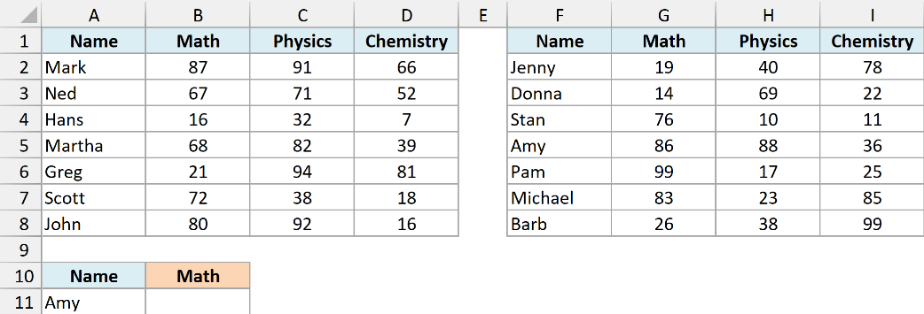
Below is the nested XLOOKUP formula that will check for the name in both the tables and return the corresponding value from the specified column.
=XLOOKUP(A11,A2:A8,B2:B8,XLOOKUP(A11,F2:F8,G2:G8))
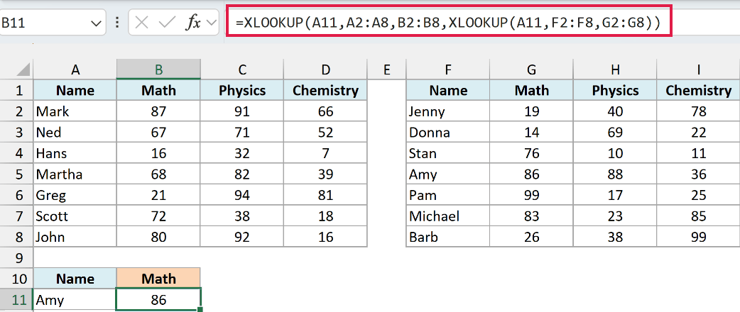
In the above formula, I have used the [if_not_found] argument to use another XLOOKUP formula. This allows you to add the second XLOOKUP in the same formula and scan two tables with a single formula.
I am not sure how many nested XLOOKUPs you can use in a formula. I tried till 10 and it worked, then I gave up 🙂
Example 6: Find the Last Matching Value
This one was badly needed and XLOOKUP made this possible. Now you don’t need to find convoluted ways to get the last matching value in a range.
Suppose you have the dataset as shown below and you want to check when was the last person hired in each department and what was the hire date.
The rows must be ordered from earliest to latest hire date for the last matching row to represent the latest hire.

The below formula will lookup the last value for each department and give the name of the last hire:
=XLOOKUP(F1,$B$2:$B$15,$A$2:$A$15,,,-1)
And the below formula will give the hire date of the last hire for each department:
=XLOOKUP(F1,$B$2:$B$15,$C$2:$C$15,,,-1)

Since XLOOKUP has an inbuilt feature to specify the direction of the lookup (first to last or last to first), this is done with a simple formula. With vertical data, VLOOKUP and INDEX/MATCH always look from top to bottom, but with XLOOKUP you can specify the direction as bottom to top as well.
Example 7: Approximate Match with XLOOKUP (Find Commission Rate)
Another notable improvement with XLOOKUP is that now there are four match modes (VLOOKUP has 2 and MATCH has 3).
You can specify any one of these four match_mode values to decide how the lookup value should be matched:
- 0 – Exact match, where the lookup_value should exactly match the value in the lookup_array. This is the default option.
- -1 – Looks for the exact match, but if it isn’t found, returns the next smaller item/value
- 1 – Looks for the exact match, but if it isn’t found, returns the next larger item/value
- 2 – To do partial matching using wildcards (* or ?), with ~ to escape a literal wildcard
But the best part is that with the default search mode, you don’t need to worry whether your data is sorted. If you switch to binary search mode (2 or -2), the lookup array must be sorted in the matching direction.
Below I have a dataset where I want to find the commission of each person, and the commission needs to be calculated using the table on the right.

Below is the formula that will do this:
=XLOOKUP(B2,$E$2:$E$6,$F$2:$F$6,0,-1)*B2

This simply uses the sales value as the lookup and looks through the lookup table on the right. In this formula, I have used -1 as the fifth argument ([match_mode]), which means that it will look for an exact match, and when it doesn’t find one, it will return the value just smaller than the lookup value.
And as I said, with this default search mode, you don’t need to worry whether your data is sorted or not.
Follow along with the example file
XLOOKUP Function Examples.xlsx
Example 8: Horizontal Lookup
XLOOKUP can do vertical as well as a horizontal lookup.
Below I have a dataset where I have student names and their scores in rows, and I want to fetch the score for the name in cell B6.

The below formula will do this:
=XLOOKUP(B6,B1:O1,B2:O2)

This is nothing but a simple lookup (similar to what we saw in Example 1), but horizontal.
All the examples that I cover about vertical lookup can also be done with a horizontal lookup using XLOOKUP (farewell to VLOOKUP and HLOOKUP).
Example 9: Conditional Lookup (Using XLOOKUP with Other Formulas)
This one is a slightly advanced example, and also shows the power of XLOOKUP when you need to do complex lookups.
Below is a data set where I have the names of students and their scores, and I want to know the name of the student who has scored the maximum in each subject and the count of students who have scored more than 80 in each subject.
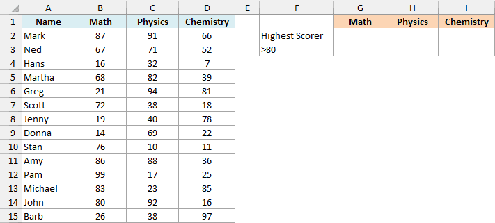
Below is the formula that will give the name of the student with the highest marks in each subject:
=XLOOKUP(MAX(XLOOKUP(G1,$B$1:$D$1,$B$2:$D$15)),XLOOKUP(G1,$B$1:$D$1,$B$2:$D$15),$A$2:$A$15)
Since XLOOKUP can be used to return an entire array, I have used it to first get all the marks for the required subject.
For example, for Math, when I use XLOOKUP(G1,$B$1:$D$1,$B$2:$D$15), it gives me all the scores in math. I can then use the MAX function to find the maximum score in this range.
This maximum score then becomes my lookup value, and the lookup range would be the array returned by XLOOKUP(G1,$B$1:$D$1,$B$2:$D$15)
I use this within another XLOOKUP formula to fetch the name of the student who has scored the maximum marks.
And to count the number of students who have scored more than 80, use the below formula:
=COUNTIF(XLOOKUP(G1,$B$1:$D$1,$B$2:$D$15),">80")
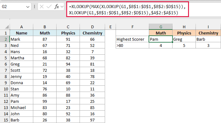
This one simply uses the XLOOKUP formula to get a range of all the values for the given subject. It then wraps it in COUNTIF function to get the number of scores that are more than 80.
Example 10: Using Wildcard in XLOOKUP
Just like you can use wildcard characters in VLOOKUP and MATCH, you can also do this with XLOOKUP.
But there is a difference.
In XLOOKUP, set the fifth argument to 2 for wildcard matching. Otherwise, the default exact-match mode treats those symbols literally and returns #N/A only if that literal lookup text is missing.
Below is a dataset where I have company names and their market capitalization.
The market-cap figures in this example and the next are illustrative values for showing how the formulas work, not current market data.

I want to look up a company name in column D, and fetch the market capitalization from the table on the left. And since the names in Column D are not exact matches, I will have to use wildcard characters.
Below is the formula that will do this:
=XLOOKUP("*"&D2&"*",$A$2:$A$11,$B$2:$B$11,,2)

In the above formula, I have used asterisk (*) wildcard character before and after D2 (it needs to be within double quotes and joined with D2 using ampersand).
This tells the formula to look through all the cells, and if it contains the word in cell D2 (which is Apple), consider it a match. No matter how many and what characters are before and after the text in cell D2.
And to make sure XLOOKUP accepts wildcard characters, the fifth argument has been set to 2 (wildcard character match).
Example 11: Find the Last Value in the Column
Since XLOOKUP allows you to search from bottom to top, you can find the last text match in a list with the wildcard formula below, as well as fetch the corresponding value from another column.
Suppose you have a dataset as shown below and you want to know what’s the last company and what’s the market capitalization of this last company.

The below formula will give you the name of the last company:
=XLOOKUP("*",A2:A11,A2:A11,,2,-1)
And the below formula will give the market cap of the last company in the list:
=XLOOKUP("*",A2:A11,B2:B11,,2,-1)

These formulas again use wildcard characters. The asterisk (*) matches text, so numbers are skipped. It also matches empty text returned by a formula such as =””, so this is not a general last-nonblank lookup.
And since the direction is from bottom to top (for the vertically arranged data), it will return the last text match in the list.
And the second formula uses a separate return_array (B2:B11) to get the market cap of the last company in the list.
Follow along with the example file
XLOOKUP Function Examples.xlsx
Example 12: Look to the Left
One of the biggest limitations of VLOOKUP is that it can only look to the right of the lookup column. XLOOKUP has no such limit, so a left lookup is just as easy as any other.
In the dataset below, the employee names are in column B and their IDs are in column A, to the left. I want to find an employee’s ID using their name.
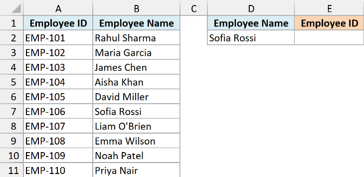
Here is the formula:
=XLOOKUP(D2,B2:B11,A2:A11)
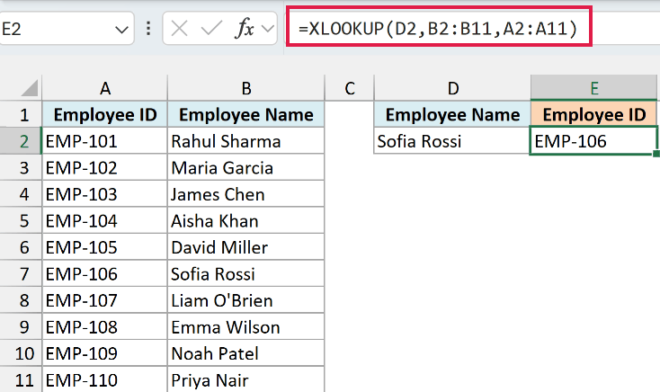
XLOOKUP finds the name in the lookup array (column B) and returns the matching ID from the return array (column A), even though it sits to the left. With VLOOKUP you would need INDEX/MATCH or a rearranged table to do the same thing.
Why Your XLOOKUP Formula Isn’t Working
If XLOOKUP is throwing an error or giving you the wrong result, it is almost always one of these:
- #NAME? error: your version of Excel doesn’t have XLOOKUP. It’s only in Microsoft 365, Excel 2021, Excel 2024, and the web. In Excel 2019 and earlier the formula shows up as _xlfn.XLOOKUP.
- #N/A error: the lookup value isn’t found. Check for extra spaces (wrap the lookup value in TRIM), or add the if_not_found argument to return a friendly message instead.
- Wrong result or #VALUE! error: your lookup_array and return_array are different sizes. They need the same number of rows (or columns for a horizontal lookup).
- #SPILL! error: XLOOKUP is returning more than one cell and something is blocking the spill range. Clear the cells next to the formula.
- A number won’t match: a lookup value of 100 won’t match “100” stored as text. Make both the same type.
XLOOKUP Frequently Asked Questions
Is XLOOKUP better than VLOOKUP?
For most lookups, yes. XLOOKUP can look to the left, returns an exact match by default, handles “not found” with a built-in argument, and can spill an entire row or column. VLOOKUP is still fine for simple right-side lookups, especially in older versions of Excel that don’t have XLOOKUP.
Does XLOOKUP work in Excel 2016 or 2019?
No. XLOOKUP is only available in Microsoft 365, Excel 2021, Excel 2024, and Excel for the web. In Excel 2016 and 2019 you’ll need to use VLOOKUP, HLOOKUP, or the INDEX/MATCH combo.
Does XLOOKUP do an exact match by default?
Yes. Unlike VLOOKUP, XLOOKUP looks for an exact match automatically, so you don’t have to remember to add FALSE or 0 at the end of the formula.
Can XLOOKUP look to the left?
Yes. XLOOKUP works in any direction, so the return column can sit to the left of the lookup column. This is one of the main reasons people switch from VLOOKUP.
So these are 12 XLOOKUP examples that can help you get your lookup and reference work done faster.
Hope you found this tutorial useful!
You may also like the following Excel tutorials:
- How to Compare Two Excel Sheets (for differences)
- Excel LAMBDA Function
- How to Compare Two Columns in Excel (for matches & differences)
- Find the Last Occurrence of a Lookup Value a List in Excel
- Lookup the Second, the Third, or the Nth Value in Excel
- Excel TAKE Function
- LOOKUP Function in Excel
- SWITCH in Excel
