How to Fix the #SPILL! Error in Excel

To fix the #SPILL! error in Excel, you need to find out what’s stopping your formula from filling the cells it needs, and then remove that obstacle. Most of the time, it’s something small sitting in the way.

In this article, I’ll show you the common reasons you get this error and how to fix each one. For every reason, you’ll see the formula failing first and then the version that works.

What Does the #SPILL! Error Mean in Excel?

A spilling formula is one formula that returns several results. You enter it in one cell, and Excel fills the nearby cells with the rest of the results.

The cells it fills are called the spill range.

The #SPILL! error comes from spilling formulas, which work in Excel 365, Excel 2024, Excel 2021, and Excel for the web.

Below I have a list of bakery items, and I’ve entered the same formula in D2, F2, and H2 to get the unique items, using the UNIQUE function:

=UNIQUE(A2:A11)

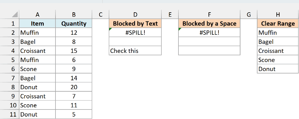
In column H, the formula filled H2:H6 with the five unique items. In D2 and F2, the same formula shows the #SPILL! error, because something in those columns is in the way.

You get the #SPILL! error when Excel can’t fill the spill range. The formula itself is usually fine, and the problem is in the cells around it.

Excel also tells you what the problem is. Here are the steps to see the reason:

1. Select the cell with the #SPILL! error. Excel draws a dashed border around the range the formula wants to use, and you’ll see a small green triangle in the top-left corner of the cell.

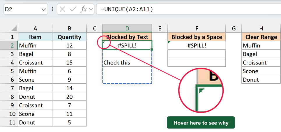
2. Hover over that green triangle. The card that appears shows the reason at the top, with the Select Obstructing Cells option below it.

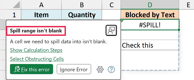
If your version of Excel shows a small warning icon next to the cell instead, click that icon. Microsoft calls this icon the error checking alert, and its menu has the same reason and the same Select Obstructing Cells option.

You can also get #SPILL! in a formula that has nothing in its way. This happens when it refers to the results of another formula that can’t spill.

For example, =SUM(D2#) adds up everything the formula in D2 spills, because the # sign after D2 means its whole spill range. If D2 shows #SPILL!, this formula shows #SPILL! too, so fix D2 first and the other one recovers on its own.

Fix the #SPILL! Error When the Spill Range Isn’t Blank

This is the first thing to check. Excel won’t overwrite anything already in the spill range, so a single value anywhere in that range stops the entire formula.

Below I have a list of bakery items with a note in D4, and I want the unique items in column D.

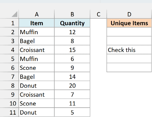
Here is the formula I entered in D2:

=UNIQUE(A2:A11)

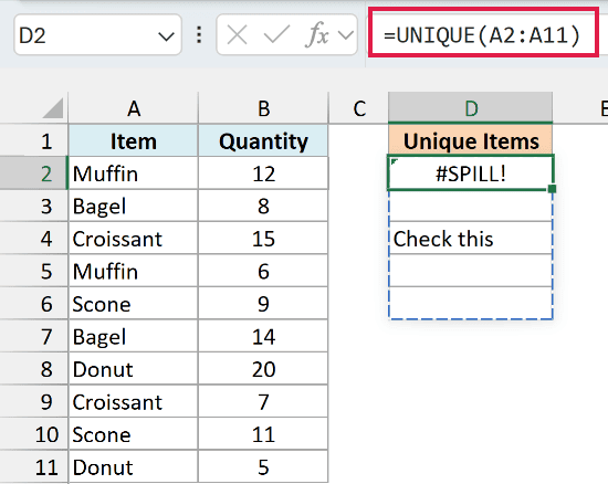
The formula needs D2:D6 for its five results, but D4 has the note in it, so all I get is #SPILL! in D2.

Here are the steps to find and clear what’s in the way:

1. Select cell D2, hover over the green triangle in its corner, and click Select Obstructing Cells. Excel selects D4.

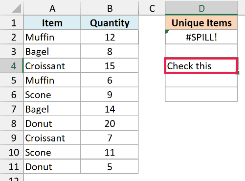
2. Press the Delete key. The formula spills right away.

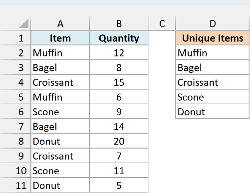
If you need to keep what’s in the cell, move it somewhere outside the spill range instead of deleting it.

When the Range Looks Empty but You Still Get #SPILL!

Sometimes every cell in the dashed border looks empty and the error still won’t go away. This happens because a cell can hold something you can’t see.

Below is the same bakery list, and I want the unique items in column F. Cell F4 looks empty, but it has a single space in it.

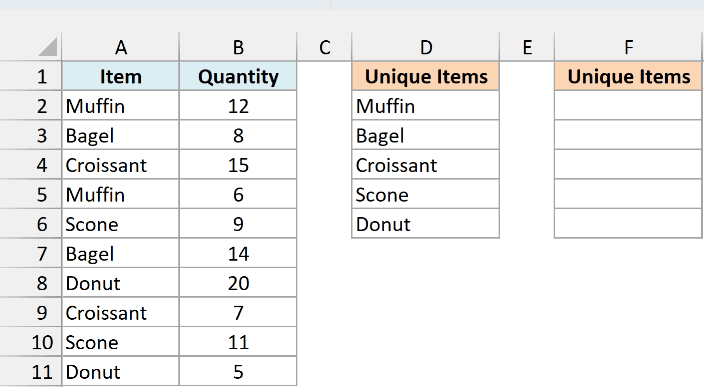
Here is the formula I entered in F2:

=UNIQUE(A2:A11)

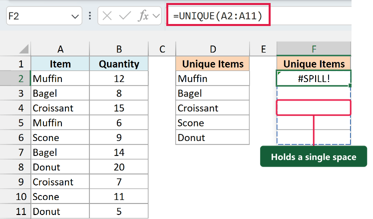
That one space is enough to block the formula. A formula returning empty text (=""), white text on a white cell, and a ;;; number format that hides the value all block it the same way.

So don’t try to spot these by eye. Use Select Obstructing Cells to jump to the cell, and then press the Delete key.

The #SPILL! Error Appears After Your Data Grows

This is the one that can catch you off guard, because the formula worked fine earlier and you never touched it. A result can grow when your data changes, and it can grow into a cell that used to be out of the way.

Below is a list of bakery orders with a note in E5, and I want all the Bagel orders in columns E:G.

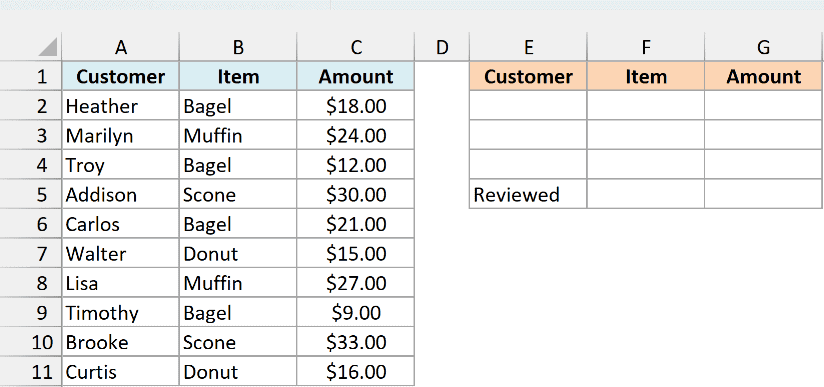
Here is the formula I entered in E2:

=FILTER(A2:C11,B2:B11="Bagel")

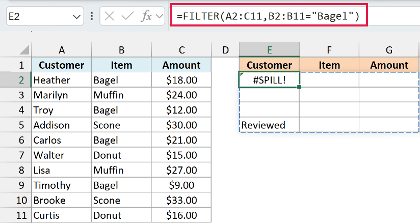
Let’s suppose this list used to have only three Bagel orders. The result fit in E2:G4, and the note in E5 caused no trouble.

Now there’s a fourth Bagel order, so the result needs E2:G5, and the note is in the way. To fix this, move the note out of those columns, and the result spills.

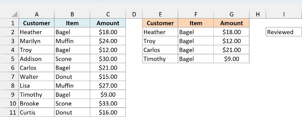
In the example file, I2 has the same FILTER formula with nothing in its way, so you can compare the two.

Since the result of the FILTER function can keep growing, it’s best to keep the cells below it empty. Put your notes above the result or in a column it will never reach.

Fix #SPILL! Caused by Merged Cells

A spilling formula can’t put results into a merged cell, even an empty one. It also can’t spill when the formula’s own cell is merged.

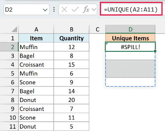
Below is a list of bakery items with a merged cell in D4:D5 (I’ve shaded it gray so you can see it), and I want the unique items in column D.

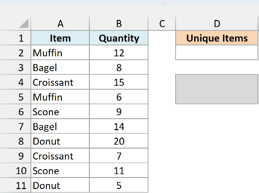
Here is the formula I entered in D2:

=UNIQUE(A2:A11)

Here are the steps to unmerge the cell:

1. Select the merged cell D4:D5.

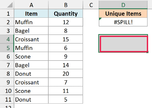
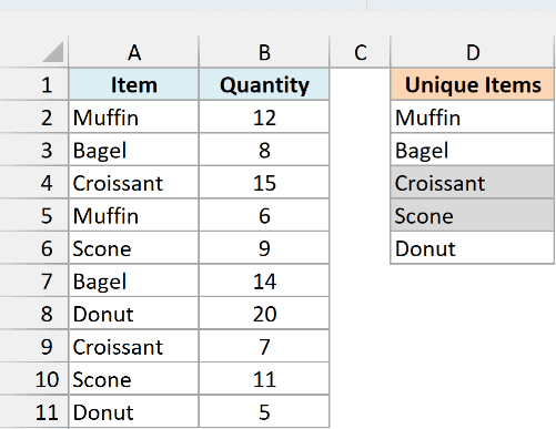
2. Click the Home tab, and then click Merge & Center. The cells unmerge and the formula spills.

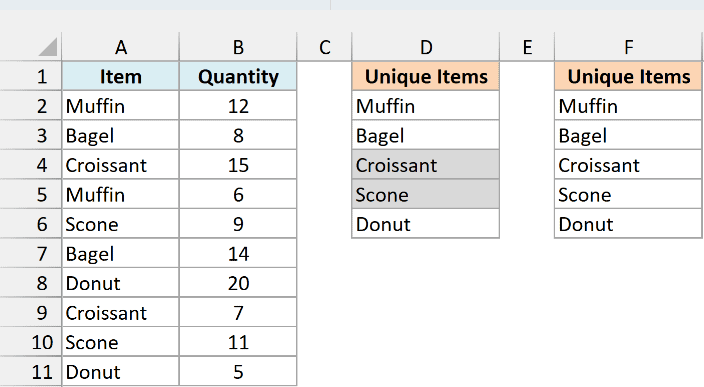
The fix is the same when the formula itself sits in a merged cell. In the example below, F2:F3 is merged and has the same formula in it, so it shows #SPILL! even though every cell below it is empty.

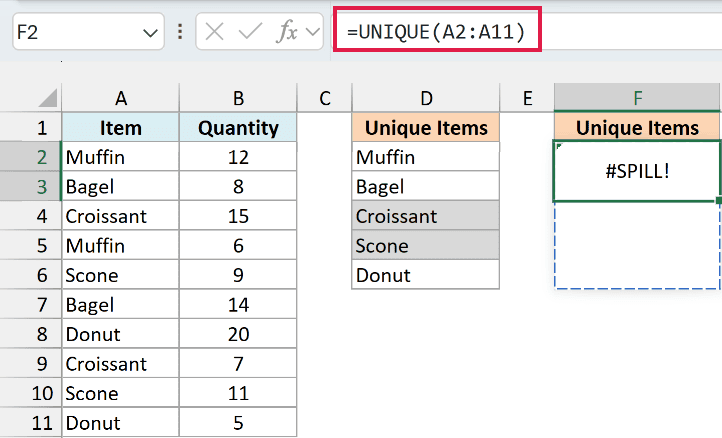
Select F2:F3 and click Merge & Center to unmerge it, and the formula spills from F2.

Fix #SPILL! in an Excel Table

Excel Tables don’t allow spilling formulas, because each cell in a Table column has to hold its own single result. So a formula that returns several results shows #SPILL! in a Table.

Below is an Excel Table named BakeryOrders with the quantity and price of each item, and I want the total for each item in column D.

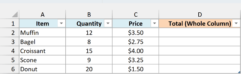
Here is the formula I entered in D2:

=[Quantity]*[Price]

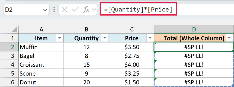
Here, [Quantity] and [Price] refer to the entire columns, so the formula returns five results. A Table can’t spill them, and since Excel fills a Table formula down the column, every row shows the error.

Important: Converting this Table to a normal range doesn’t fix the #SPILL! in column D on its own. The copies of the formula in D3:D6 stay there and block the spill, so you need to clear them too.

The fix is to ask for the value in the current row only, which is what the @ sign does. Here is the formula that works, which I’ve entered in column E:

=[@Quantity]*[@Price]

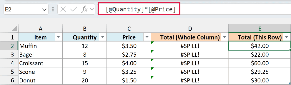
Now each row multiplies its own quantity and price, and Excel fills the formula down the whole column for you.

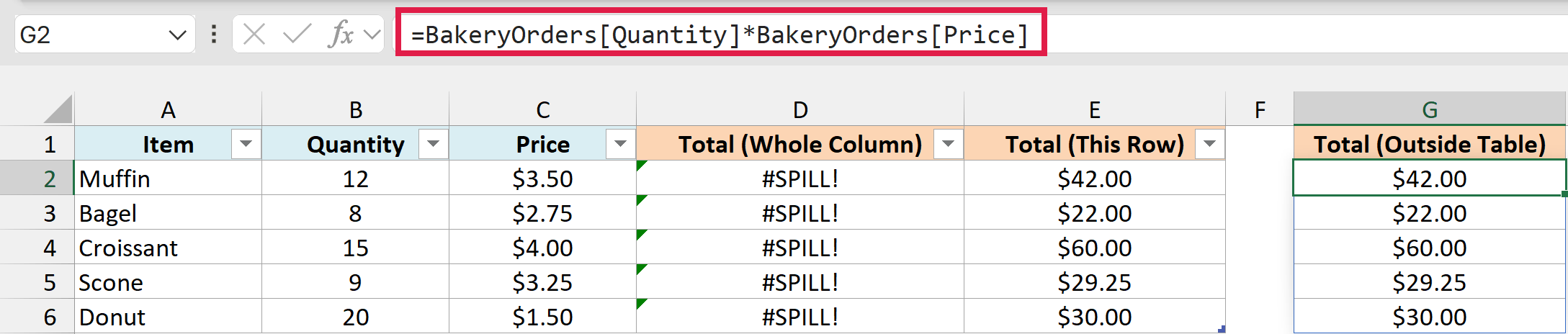
If you do want one spilling formula, enter it outside the Table. Here is the formula I entered in G2, which refers to the same Table columns:

=BakeryOrders[Quantity]*BakeryOrders[Price]

Fix #SPILL! When the Spill Range Is Too Big

A formula also fails when its results won’t fit on the worksheet. This usually happens when you refer to an entire column as the value to look up.

Below I have a price list and a few items to find, and I want the price of each item in column E.

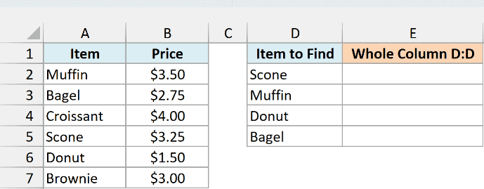
Here is the formula I entered in E2:

=XLOOKUP(D:D,A2:A7,B2:B7)

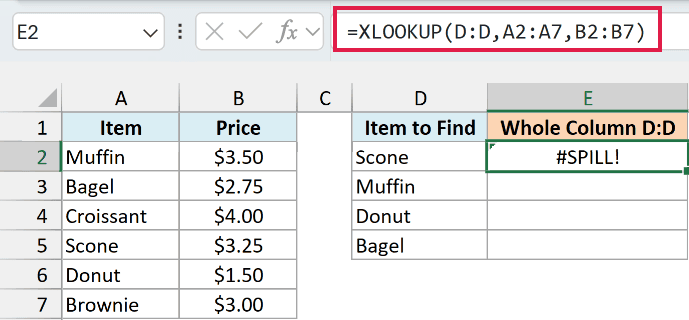
D:D has 1,048,576 cells, so the XLOOKUP function tries to return 1,048,576 results. Starting from E2, there are only 1,048,575 rows left, so the results don’t fit.

The same thing happens with VLOOKUP when its lookup value is a whole column.

To fix this, refer only to the cells that have your lookup values. Here is the formula I entered in F2:

=XLOOKUP(D2:D5,A2:A7,B2:B7)

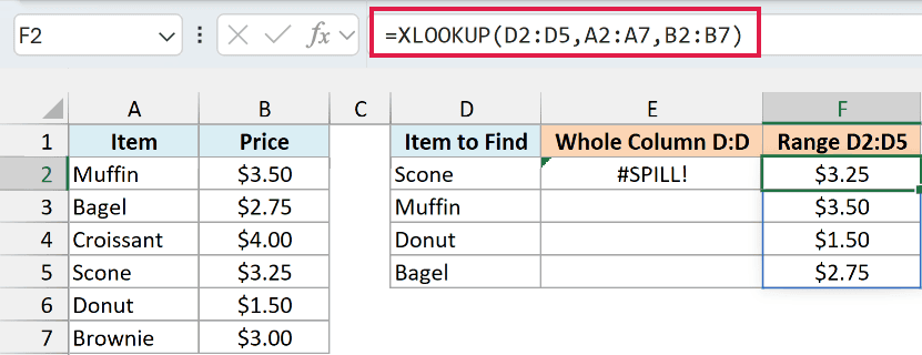
Now XLOOKUP has only four values to look up, so it spills four prices.

If you don’t want the formula to spill at all, look up one cell at a time. Here is the formula I entered in G2 and copied down to G5:

=XLOOKUP(D2,$A$2:$A$7,$B$2:$B$7)

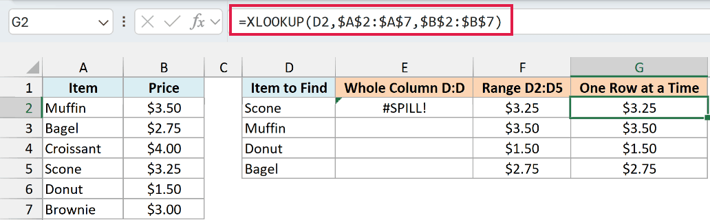
I’ve used absolute references for the price list so that it stays in place when you copy the formula down.

You may also see an @ sign in formulas such as =XLOOKUP(@D:D,A2:A7,B2:B7). It tells Excel to use only the value from the formula’s own row (D2 for a formula in E2), so the formula returns one result, like the copied-down version above.

This isn’t a general fix though. If the formula sits in a row outside the range it refers to, such as =XLOOKUP(@D2:D5,A2:A7,B2:B7) in E7, you get the #VALUE! error instead.

Fix #SPILL! When the Result Size Keeps Changing

This one is less common and a bit odd. Functions such as RANDBETWEEN give a new number every time Excel recalculates, so a result sized by RANDBETWEEN keeps changing height, and Excel can’t always settle on it.

Below I want a list of ticket numbers in column D, and I want the number of tickets to be random.

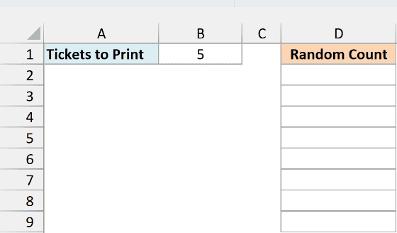
Here is the formula I entered in D2, which uses the SEQUENCE function with a random count between 3 and 8:

=SEQUENCE(RANDBETWEEN(3,8))

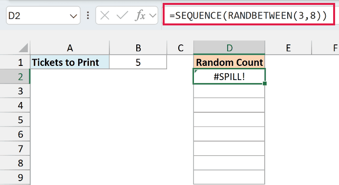
This error is random. In my tests, the same formula spilled on some recalculations and showed #SPILL! on others, so you may see a working list when you open the example file.

To see the error, press F9 a few times or re-enter the formula in D2. I’ve added the border in D2:D9 to mark the eight rows this formula can use at most, so it isn’t the dashed border Excel draws.

Moving RANDBETWEEN into a helper cell or into the LET function didn’t stop the error in my tests. What did stop it is a count that doesn’t change.

Here is the formula I entered in F2, which uses the number of tickets I’ve typed in B1:

=SEQUENCE(B1)

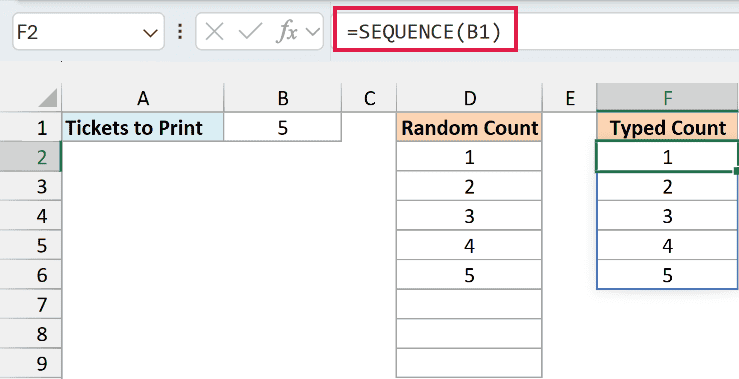
This gave me no error in 75 recalculations. If you do want a random count, generate it in another cell and paste it into B1 as a value.

Less Common Reasons for the #SPILL! Error

Microsoft lists two more reasons Excel may give you for this error. I couldn’t reproduce either one, so I’m going by Microsoft’s guide to the #SPILL! error here.

Out of memory means the formula is working with more data than Excel can handle, so try referring to a smaller range. Unrecognized means Excel can’t identify the cause, so check that the formula has all its required arguments.

So these are the reasons you get the #SPILL! error in Excel and how to fix each one. I hope you found this article helpful.

Other Excel Articles You May Also Like:

• How to Fix Excel Functions That Won’t Spill (EOMONTH, EDATE, WORKDAY)
• EXPAND Function in Excel