EXPAND Function in Excel

If you want to grow an array to a set number of rows or columns and fill the extra cells with a value of your choice, the EXPAND function is what you’re looking for.

EXPAND is a dynamic array function, so it spills its results across the cells below and to the right.

In this article, I’ll show you how to use EXPAND in Excel with a few practical examples.

EXPAND Function Syntax

Here is the syntax of the EXPAND function:

=EXPAND(array, rows, [columns], [pad_with])

• array – The range or array you want to expand.
• rows – The number of rows you want the result to have. Leave it out and the row count stays the same.
• columns – The number of columns you want the result to have. Leave it out and the column count stays the same.
• pad_with – The value that goes in the extra cells. Leave it out and Excel fills them with #N/A.

When to Use EXPAND in Excel

Use this function when you need to:

• Grow a small array to a fixed number of rows or columns.
• Fill the new cells with a specific value like 0, a dash, or a blank instead of #N/A.
• Pad a nonempty FILTER result to a fixed size, provided it doesn’t exceed that size.
• Pad a narrow table so its column count matches another table before you stack them.

Let me show you a few practical examples of how to use this function.

Example 1: Grow a Small Table to More Rows

Let’s start with a simple example.

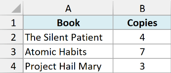
Below is the dataset. It has a small book inventory with the book title in column A and the number of copies in column B, three rows in all.

I want to display this three-row table in a six-row block. The added cells are part of the formula’s spill, so you can’t type new books into them; add records to the source and update the range instead.

Here is the formula:

=EXPAND(A2:B4,6,2)

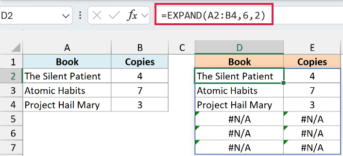
In the above formula, EXPAND takes the range A2:B4 and grows it to 6 rows and 2 columns. The three original rows stay put, and the three new rows appear below them.

Since I left out the pad_with argument, Excel fills those new cells with #N/A. That is the default, and I’ll show you how to change it in the next example.

Example 2: Pad the Extra Cells With a Value

Here’s another practical scenario.

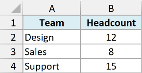
Below is the dataset. It has a headcount for three teams, with the team name in column A and the number of people in column B.

I want the headcount column to always be six rows tall so a chart built on it never changes height, and I want the empty rows to show 0 instead of #N/A.

Here is the formula:

=EXPAND(B2:B4,6,1,0)

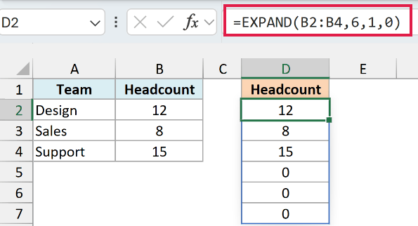
Here, EXPAND grows the single column of headcounts to 6 rows and 1 column. The fourth argument, 0, tells Excel to put a 0 in each new cell instead of the default #N/A.

The pad_with value can be anything you like. A number, some text in quotes, or a dash all work the same way.

Pro Tip: Use an empty string (“”) as the pad_with value when you want the extra cells to look blank rather than show a placeholder.

Example 3: Add More Columns to a Table

Now let’s look at something a bit more interesting.

Below is the dataset. It has a class roster with the student name in column A and two test scores in columns B and C, four students in all.

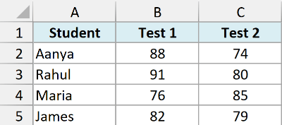
I want to display the roster with two extra blank columns. These cells are part of the spill, so you can’t enter future test scores into them; add scores to the source and update the formula instead.

Here is the formula:

=EXPAND(A2:C5,4,5,"")

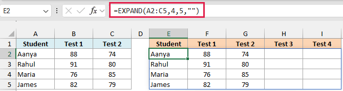
In the above formula, the array A2:C5 is 4 rows by 3 columns. I keep the rows at 4 and grow the columns to 5, so two new columns appear on the right.

The pad_with value is an empty string, so the new cells come out blank instead of showing #N/A.

Example 4: Lock a FILTER Result to a Fixed Size

Let’s step it up with a use case I reach for quite often.

Below is the dataset. It has a gym check-in list with the member name in column A and their status (Active or Inactive) in column B, eight members in all.

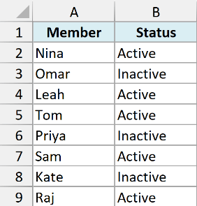
I want to pull only the active members and show them in a six-row block, provided there are between one and six active members.

Here is the formula:

=EXPAND(FILTER(A2:A9,B2:B9="Active"),6,1,"")

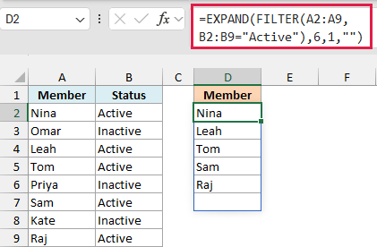
How this formula works:

• FILTER(A2:A9,B2:B9=”Active”) pulls the five active members into a spilled list.
• EXPAND then grows that list to 6 rows and 1 column, so the block stays six rows tall when FILTER returns between one and six members.
• The empty string in the pad_with slot leaves the leftover row blank.

This is handy for a dashboard, where a FILTER result that grows and shrinks would otherwise push your other elements around. Wrapping it in EXPAND keeps the footprint steady.

Pro Tip: EXPAND needs at least as many rows as FILTER returns. More than six matches gives a #VALUE! error, because EXPAND never trims. With no matches, this FILTER formula returns #CALC! because it has no if_empty argument.

Example 5: Match Column Counts Before Stacking

This last one combines EXPAND with VSTACK.

Below is the dataset. It has two small price lists side by side. The first list in columns A to C has three columns (Item, Price, Status), and the second list in columns E and F has only two (Item, Price).

I want to stack the second list under the first, and use dashes in its missing Status column. VSTACK accepts different widths, but normally fills the extra cells with #N/A.

Here is the formula:

=VSTACK(A2:C3,EXPAND(E2:F3,2,3,"-"))

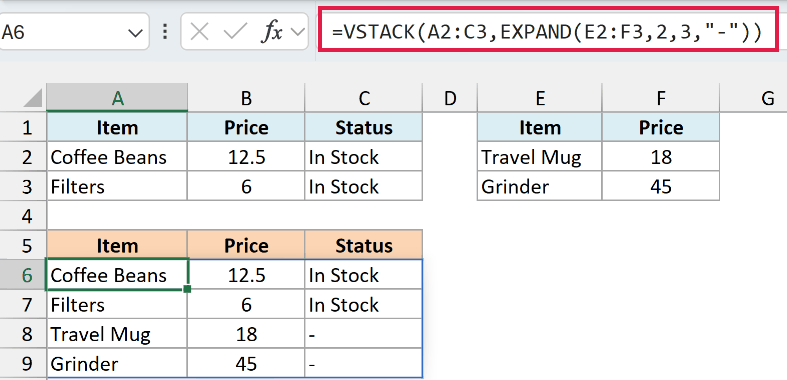
How this formula works:

• EXPAND(E2:F3,2,3,”-“) grows the two-column list to three columns, keeping its 2 rows and adding a dash in the new Status cells.
• VSTACK then stacks that padded list under the first list, and both now have three columns, so there is no size mismatch.

Without EXPAND, VSTACK would fill the missing column with #N/A. Padding it first lets you decide exactly what those cells show.

Tips & Common Mistakes

• EXPAND only grows, it never shrinks. If the rows or columns value is smaller than the array you pass in, you get a #VALUE! error. To pull a set number of rows off the top or bottom, use the TAKE function. To remove rows or columns instead, use the DROP function.
• Omitted dimensions keep their original size. Leaving both rows and columns empty retains the source dimensions, so nothing grows.
• EXPAND grows down and to the right only. There is no built-in way to add cells above or to the left. To do that, put the new rows or columns first with VSTACK or HSTACK.
• Watch the spill range. EXPAND is a dynamic array function, so its result spills. If a cell in the spill range already has something in it, you’ll see a #SPILL! error until you clear the blocking cell.
• EXPAND is a newer function. It works in Excel for Microsoft 365 and Excel 2024. It is not available in Excel 2021 or earlier.

In this article, I covered how to use EXPAND to grow an array, how to pad the new cells with a value of your choice, and how to lock a FILTER result to a fixed size.

I also showed you how to pair it with VSTACK to line up mismatched tables.

I hope you found this article helpful.

List of All Excel Functions

Other Excel Functions You May Also Like:

• SEQUENCE Function in Excel
• XLOOKUP Function in Excel
• MAP Function in Excel

Other Excel Articles You May Also Like:

• Transpose Multiple Rows into One Column
• Remove Blank Rows in Excel Using a Formula
• 20 Advanced Excel Functions and Formulas