

If you want to pull out just the rows that meet a condition, like every applicant from one department or every order above a certain amount, the FILTER function is what you want.
FILTER is a dynamic array function, which means it spills its results across the cells below automatically. You write one formula and Excel returns every matching row.
In this article, I’ll show you how to use FILTER in Excel, from a simple single-condition filter to combining conditions, filtering by a calculated value, building a live search box, returning only the columns you need, and sorting the results.
Follow along with the example file
FILTER Function Examples.xlsx
FILTER Function Syntax
Here is the syntax of the FILTER function:
=FILTER(array, include, [if_empty])
- array – The range or array of data you want to filter.
- include – A TRUE/FALSE (Boolean) array that tells FILTER which rows or columns to keep. Match its height to the data when filtering rows, or its width when filtering columns.
- [if_empty] – Optional. The value to return when nothing matches. Leave it out and FILTER shows a #CALC! error when no rows match.
FILTER works in Excel for Microsoft 365, Excel 2021, and Excel 2024, on Windows, Mac, and the web. It is not available in Excel 2019 or earlier.
When to Use the FILTER Function
Use the FILTER function when you need to:
- Pull every row that matches one or more conditions into a new list
- Build a filtered report that updates on its own when the source data changes
- Return only the specific columns you care about from the matching rows
- Feed a filtered list straight into another formula like SORT or COUNTA
Let me show you a few practical examples of how the FILTER function works.
Example 1: Filter Rows With a Single Condition
Let’s start with the most common use, pulling out every row that meets one condition.
Below is a list of job applicants. Column A has the candidate name, column B the department, column C the years of experience, column D the application status, and column E the city.
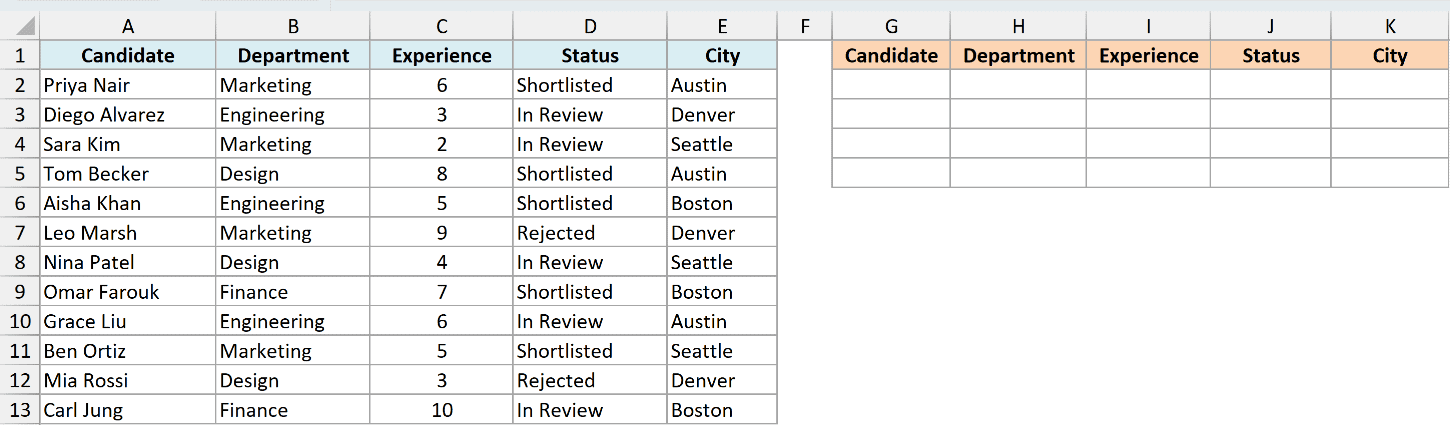
I want to pull out every applicant in the Marketing department, along with all their details.
Here is the formula:
=FILTER(A2:E13, B2:B13="Marketing")
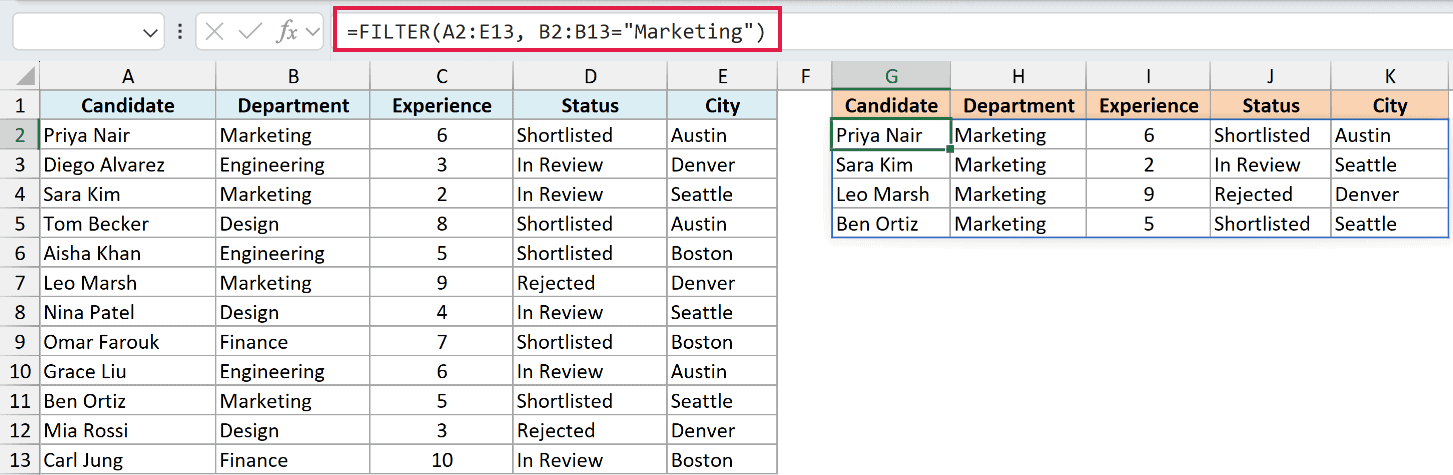
Here, the include argument B2:B13="Marketing" checks the department column and builds a TRUE/FALSE list. FILTER keeps the rows where the result is TRUE.
It then spills all five columns for those four Marketing applicants into the cells below, under the same headers and with no dragging needed.
Pro Tip: You only type this formula once, in the top-left cell. FILTER spills the rest of the rows on its own, so never drag it down or copy it across.
Example 2: Filter With Multiple Conditions Using AND
Now let’s narrow it down with two conditions that both have to be true.
I’m using the same applicants table: candidate in column A, department in column B, experience in column C, status in column D, and city in column E.
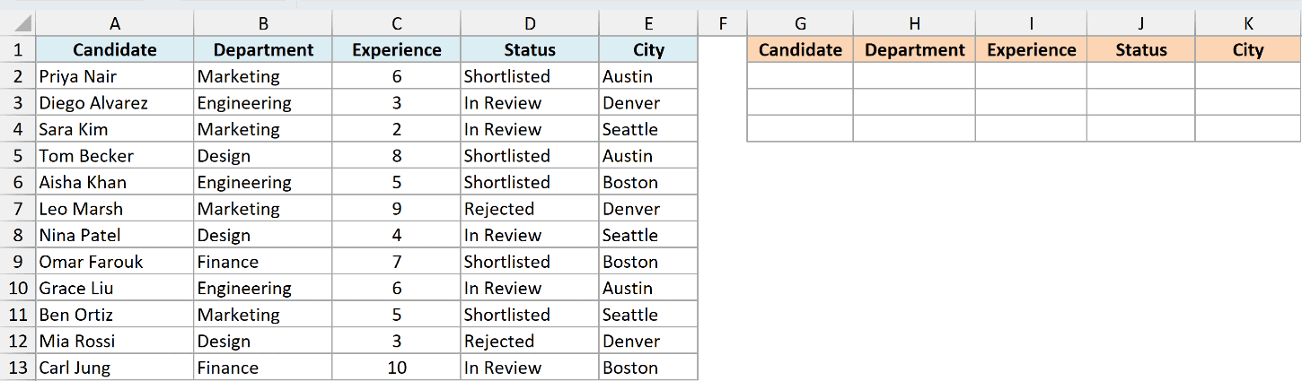
I want only the Marketing applicants who also have at least 5 years of experience.
Here is the formula:
=FILTER(A2:E13, (B2:B13="Marketing")*(C2:C13>=5))
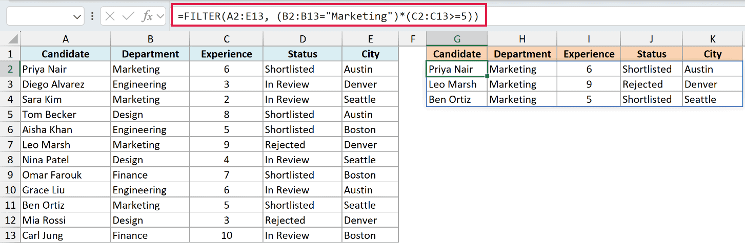
To combine conditions with AND logic, you multiply them. Each condition returns TRUE (1) or FALSE (0), and multiplying means a row only survives when both are 1.
Sara has just 2 years, so she drops out, leaving three applicants who clear both checks.
Wrap each condition in its own set of parentheses. The * between them is what creates the AND.
Example 3: Filter With Multiple Conditions Using OR
Sometimes you want rows that match either of two conditions. That is OR logic.
The dataset is the same applicants table: candidate in column A, department in column B, experience in column C, status in column D, and city in column E.
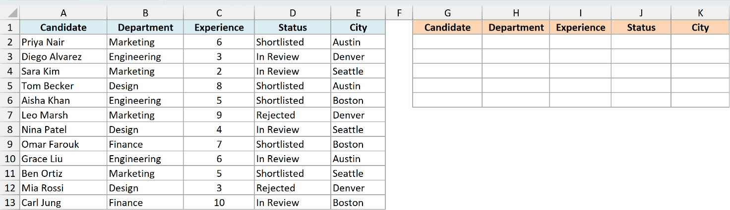
I want every applicant from either the Design or the Finance department.
Here is the formula:
=FILTER(A2:E13, (B2:B13="Design")+(B2:B13="Finance"))
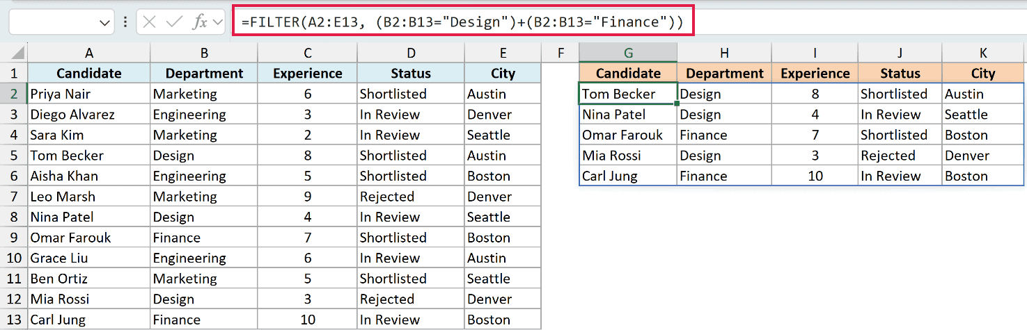
For OR logic you add the conditions instead of multiplying. A row passes when at least one condition is TRUE, so the sum comes out to 1 or more.
This returns all five Design and Finance applicants in one list.
Example 4: Filter Records Above the Average or in the Top N
Here’s a case where the cutoff isn’t a number you type in. It comes from the data itself.
I’m using the same applicants table: candidate in column A, department in column B, experience in column C, status in column D, and city in column E.
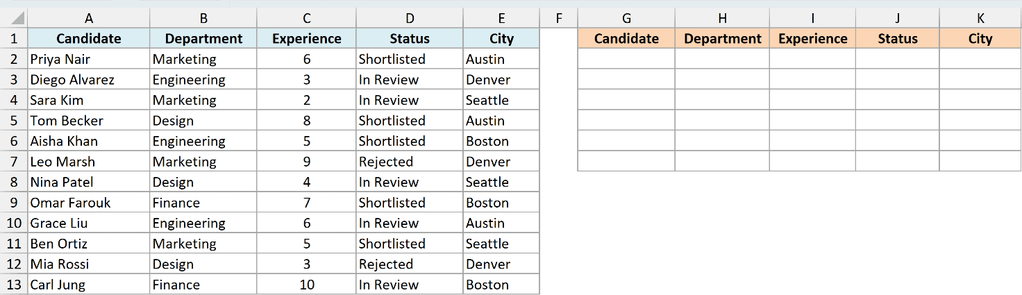
I want every applicant whose experience is above the average for the whole group.
Here is the formula:
=FILTER(A2:E13, C2:C13>AVERAGE(C2:C13))
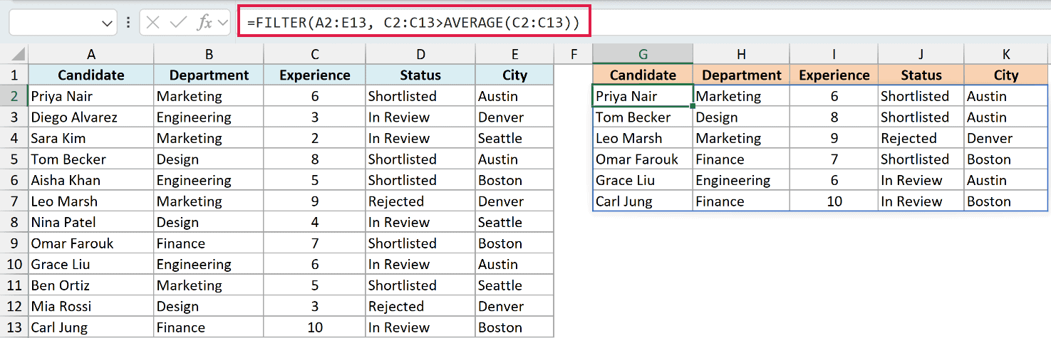
AVERAGE(C2:C13) works out the average experience first, which is about 5.7 years. FILTER then keeps only the rows where the experience beats that number.
Six applicants clear the bar, from Priya at 6 years up to Carl at 10.
Now let’s change the cutoff. Say you want only the three most experienced applicants instead.
Here is the formula:
=FILTER(A2:E13, C2:C13>=LARGE(C2:C13, 3))
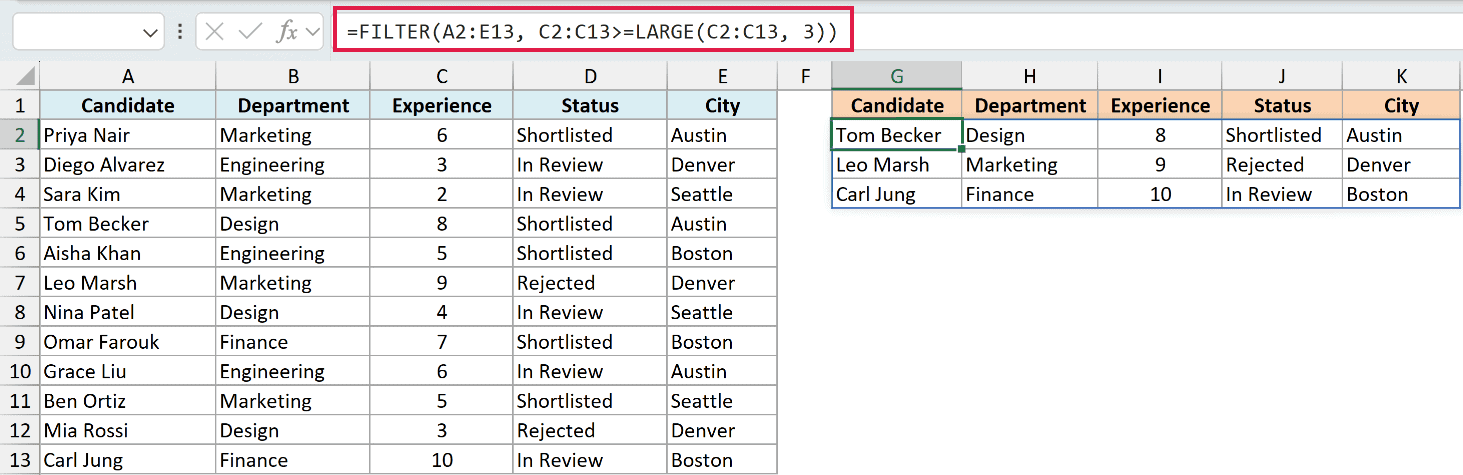
LARGE(C2:C13, 3) returns the third-largest experience value, which is 8. FILTER then keeps every row at 8 years or more, so you get Carl, Leo, and Tom.
If more applicants tie at that cutoff, this formula returns all of them, so the result can contain more than three rows.
Pro Tip: For the applicants below average, just flip the sign: =FILTER(A2:E13, C2:C13<AVERAGE(C2:C13)).
Example 5: Filter Every Other Row (Even or Odd Records)
Here’s a niche one that comes in handy more often than you’d think, pulling out every other row.
The dataset is the same applicants table, with the candidate, department, experience, status, and city in columns A through E.
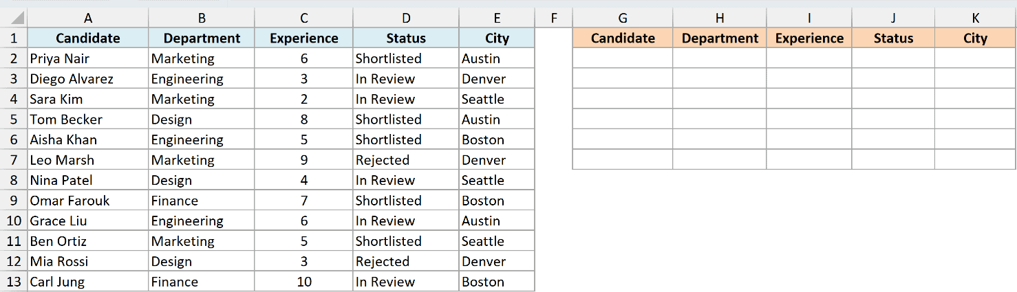
I want only the even-numbered records, so the 2nd, 4th, 6th applicant, and so on down the list.
Here is the formula:
=FILTER(A2:E13, MOD(ROW(A2:A13)-1, 2)=0)
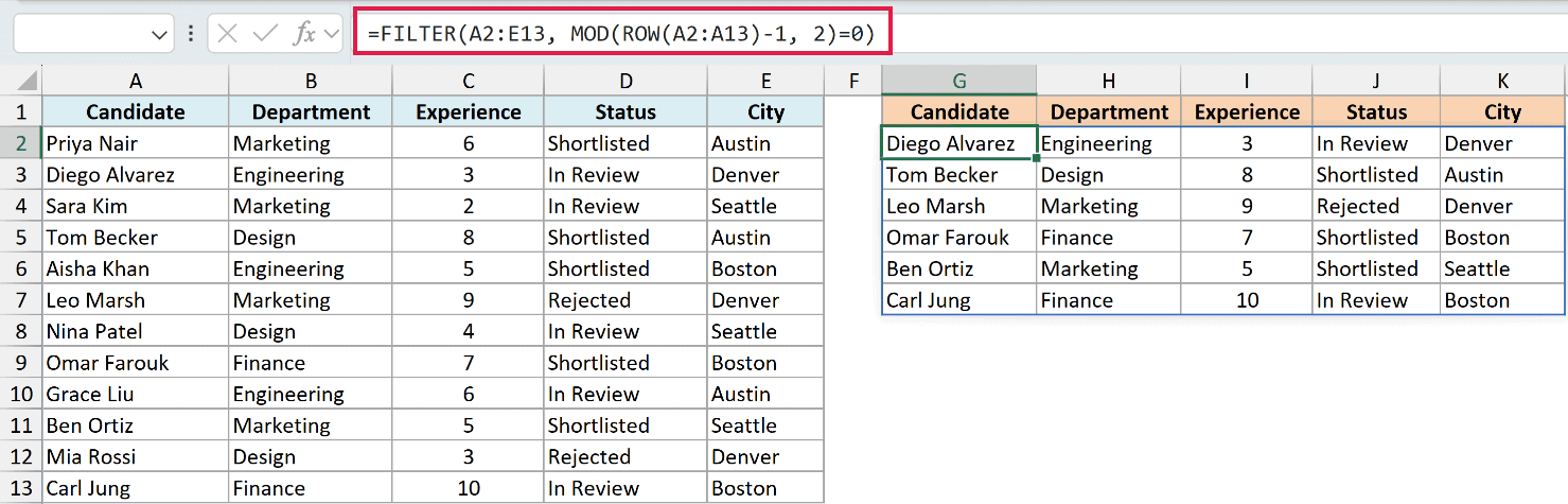
ROW(A2:A13) gives each row’s number, and subtracting 1 turns the first record into 1, the second into 2, and so on. MOD(…, 2)=0 is TRUE only for the even ones.
That returns the six even-numbered applicants, starting with Diego.
Pro Tip: For the odd-numbered records, change the 0 to a 1: =FILTER(A2:E13, MOD(ROW(A2:A13)-1, 2)=1).
Example 6: Build a Live Search Box With a Drop-Down
This is where FILTER gets really useful. You can point the condition at a cell and let anyone pick the value.
The dataset is the same applicants table, with the candidate, department, experience, status, and city in columns A through E. I’ve added a “Department” label in cell G1, with a drop-down list next to it in cell H1 that has the department names.
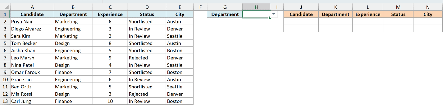
I want the filtered list to update the moment I pick a different department from that drop-down.
Here is the formula:
=FILTER(A2:E13, B2:B13=H1)
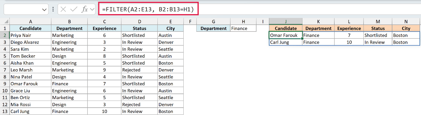
Instead of hard-coding “Marketing”, the condition now reads whatever sits in H1. Pick “Finance” from the drop-down and FILTER shows the two Finance applicants right away.
Change the selection to “Engineering” and the list refreshes on its own. That’s a working search box in a single formula, no macros needed.
Pro Tip: Build the drop-down with Data > Data Validation > List, and point it at your list of departments so nobody can mistype a name.
Example 7: Handle No Matches With the if_empty Argument
Here is the one thing that trips people up. What happens when nothing matches?
The dataset is the same applicants table, with the candidate, department, experience, status, and city in columns A through E.
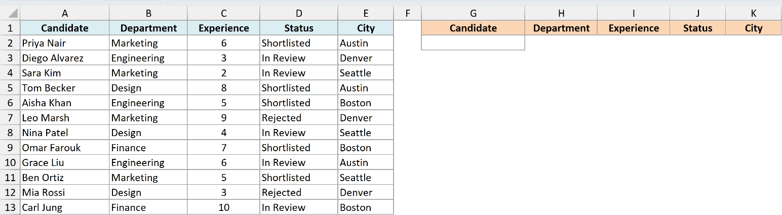
I want the applicants from the Sales department, but there aren’t any in this list.
Here is the formula:
=FILTER(A2:E13, B2:B13="Sales", "No applicants found")
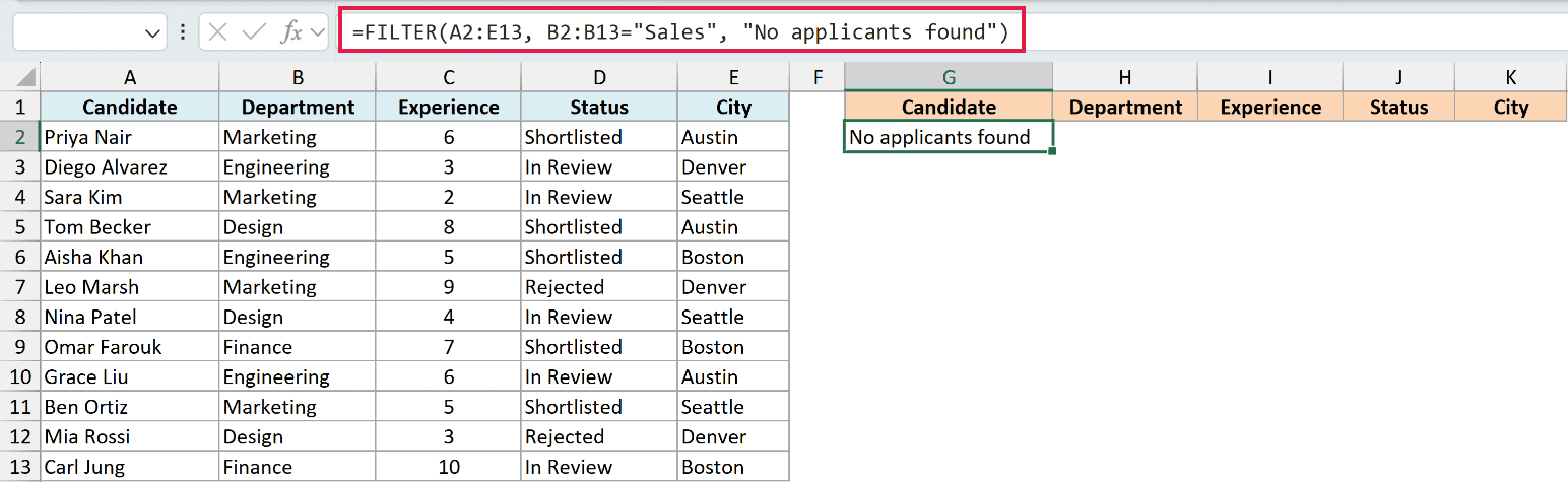
There is no Sales department in the data. Without the third argument, FILTER would return a #CALC! error here.
The if_empty argument, which is "No applicants found" in this case, gives FILTER something friendly to show instead.
Pro Tip: Get in the habit of adding an if_empty message to any FILTER whose result might come up empty. It keeps a stray #CALC! error out of your reports.
Example 8: Return Only Specific Columns
You don’t always want the whole row back. FILTER can return just the columns you care about.
The dataset is the same applicants table, with the candidate, department, experience, status, and city in columns A through E.
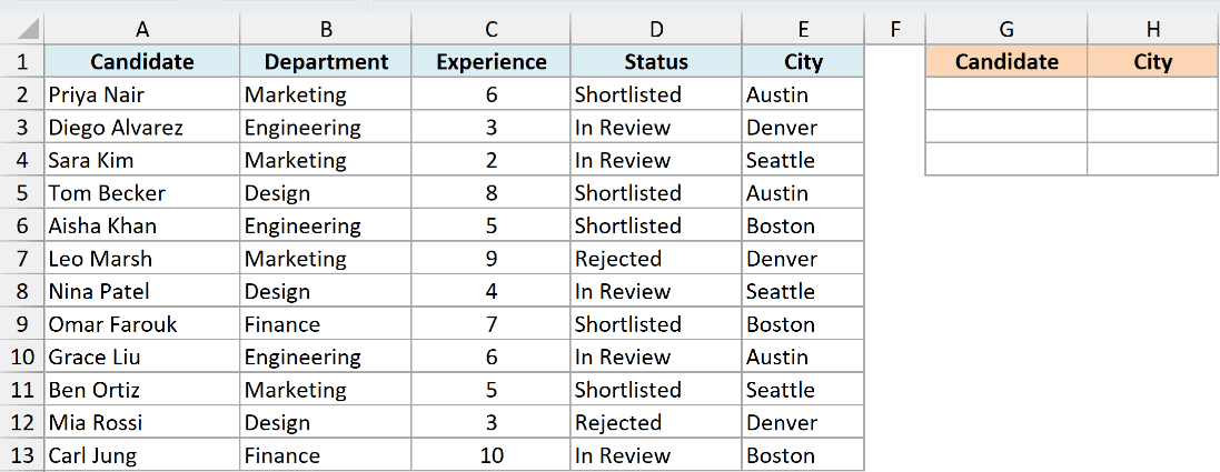
I want only the candidate name and city for everyone in the Engineering department, not the full row.
Here is the formula:
=FILTER(CHOOSECOLS(A2:E13, 1, 5), B2:B13="Engineering")
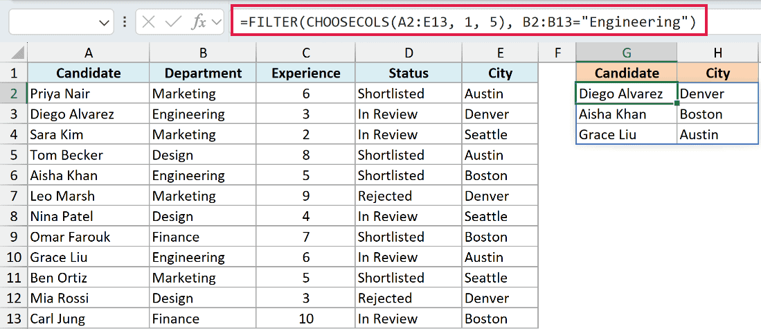
CHOOSECOLS(A2:E13, 1, 5) first trims the data down to column 1 (the candidate) and column 5 (the city).
FILTER then keeps only the Engineering rows from that trimmed data, so you end up with a clean two-column list.
Pro Tip: CHOOSECOLS needs Excel 365 or Excel 2024. In Excel 2021, filter a single column directly with =FILTER(A2:A13, B2:B13=”Engineering”), or pull the columns you want with INDEX.
Example 9: Sort a Filtered Result
You can drop FILTER straight inside other dynamic array functions. A common pairing is SORT.
The dataset is the same applicants table, with the candidate, department, experience, status, and city in columns A through E.
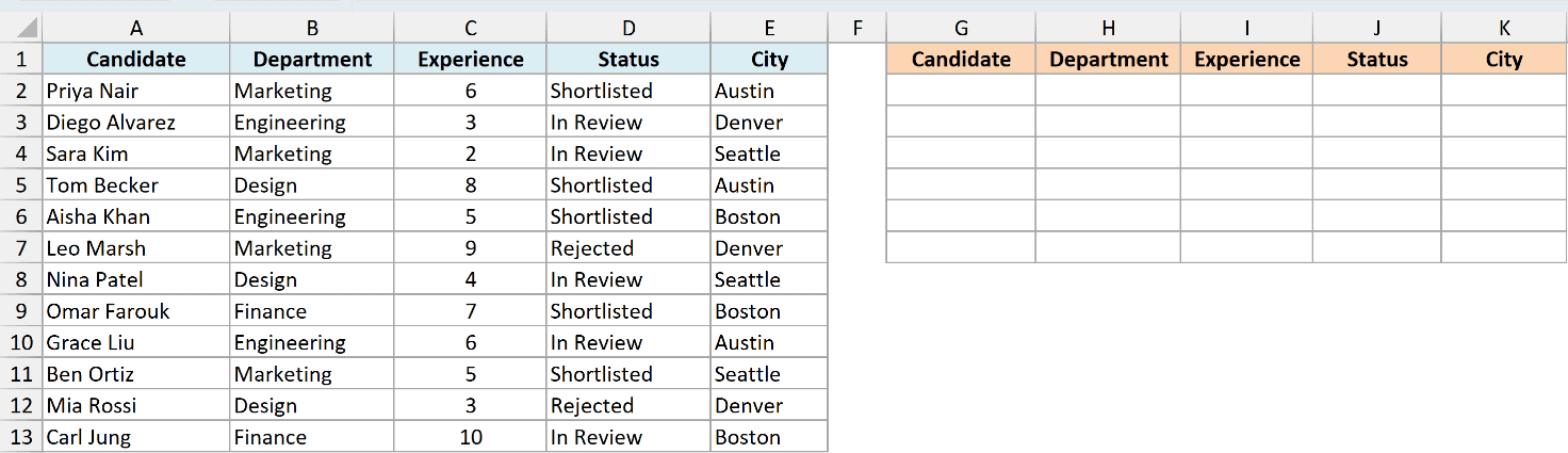
I want the applicants with 6 or more years of experience, sorted from most experienced to least.
Here is the formula:
=SORT(FILTER(A2:E13, C2:C13>=6), 3, -1)
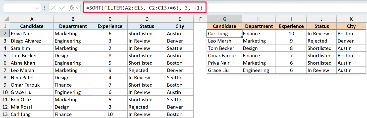
FILTER runs first and returns everyone with 6 or more years. SORT then orders that result by column 3, which is the experience column.
The -1 tells SORT to go largest to smallest, so Carl’s 10 years lands right on top.
Example 10: Reuse a Filtered Result With the Spill Reference
Once FILTER spills a result, you can point other formulas at it without retyping the range.
The dataset is the same applicants table, with the candidate, department, experience, status, and city in columns A through E.
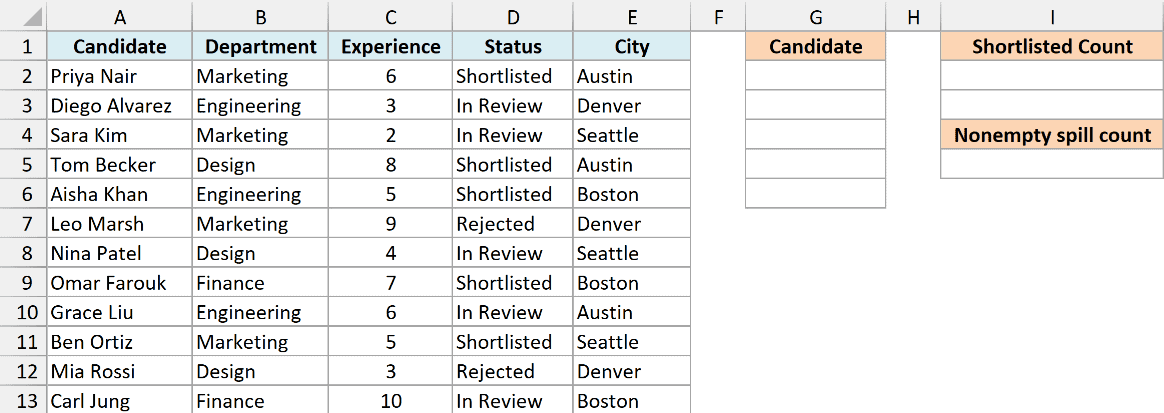
First I want a list of every shortlisted applicant, then a quick count of how many there are.
Here is the formula that pulls the list:
=FILTER(A2:A13, D2:D13="Shortlisted")
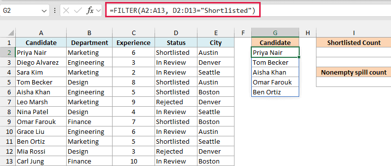
This spills the names of the five shortlisted applicants down the column, starting in cell G2.
Because the result spills, you can reference the whole range with G2#, the cell address plus a hash. Here is the count:
=COUNTA(G2#)
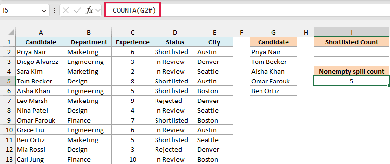
The # after G2 means “the entire spilled range that starts here.” COUNTA counts all five names for you.
COUNTA also counts an empty-string fallback or an error, so it can return 1 when nobody is shortlisted. To count applicants reliably, use =COUNTIF(D2:D13,"Shortlisted"), which returns 0 when there are no matches.
If the filter later returns more or fewer people, this count updates on its own. You can feed G2# into SORT, UNIQUE, or any other function the same way.
Tips & Common Mistakes
- #CALC! error when nothing matches. If no rows meet your condition and you skipped the if_empty argument, FILTER returns #CALC!. Add a third argument like “No matches” to handle it cleanly.
- #SPILL! error when the result is blocked. FILTER needs empty cells below and to the right to spill into. If anything is in the way, you get #SPILL!. Clear those cells and the result appears.
- You can’t edit one cell of the result. The spilled output is a single dynamic array, so you can’t change or delete an individual cell in it. Edit the formula in the top-left cell instead, and the whole result updates.
- Multiply for AND, add for OR. Use
*between conditions when every one must be true, and+when any one can be true. Wrap each condition in its own parentheses. - The include array must line up with the data. For row filtering, use a condition with the same height as the data. For column filtering, use a condition with the same width.
- FILTER is not case sensitive. “marketing” and “Marketing” match the same rows. If you need a case-sensitive match, combine FILTER with the EXACT function.
- Older versions don’t have FILTER. In Excel 2019, 2016, or earlier, use Advanced Filter or the built-in AutoFilter instead.
The FILTER function is one of the most useful additions to modern Excel. Once you’re comfortable with the include argument and the * and + operators, you can pull almost any subset of your data with a single formula.
Try it on your own data. Start with one condition, then layer on more as you need them.
Other Excel Articles You May Also Like:
