TRANSPOSE Function in Excel

If you want to turn rows into columns or columns into rows, the TRANSPOSE function in Excel flips the data for you.

In Excel 365, TRANSPOSE is a dynamic array function, so you enter it in one cell and the flipped result spills into the cells around it.

In this article, I’ll show you how to use the TRANSPOSE formula with six examples, starting with a list and working up to a summary.

Excel TRANSPOSE Function Syntax

Here is the syntax of the TRANSPOSE function:

=TRANSPOSE(array)

• array is the required range or array whose rows and columns you want to switch. It can be a plain cell range or the result of another formula.

There is only one argument. Give the TRANSPOSE function a column and it returns a row. Give it a row and it returns a column.

With a whole block, the first row becomes the first column, the second row becomes the second column, and so on. The order stays the same.

The dimensions swap too. A source with 5 rows and 4 columns returns a result with 4 rows and 5 columns.

You can also flip the result of another formula. Later examples show this with the FILTER, XLOOKUP, and UNIQUE functions.

The TRANSPOSE function returns a live result. When your source data changes, the flipped copy updates by itself.

For a fixed copy, use Paste Special with the Transpose option instead.

In Excel 365, 2024, and 2021, enter the formula in the top-left result cell and press Enter. Excel fills the rest of the output area automatically.

Important: In Excel 2019 and earlier, select the full output range first, with rows and columns swapped. Type the formula, then press Ctrl+Shift+Enter.

Excel adds the curly braces around the formula itself. Don’t type them. Pressing only Enter in those versions gives a #VALUE! error or just the first value.

TRANSPOSE is available in Excel 365, 2024, 2021, 2019, 2016, and earlier versions, as well as Excel for Mac and Excel on the web.

When to Use the TRANSPOSE Function

Use this function when you need to:

• Turn a column into a row, or a row into a column.
• Flip a whole table so rows become columns, including the headers.
• Keep the flipped copy linked to the source so it updates. Use Paste Special when you want a fixed copy.
• Rotate the output of FILTER, XLOOKUP, or UNIQUE to fit your layout.
• Build a header row from a list.

Let me show you a few practical examples of how this works.

Example 1: Convert a Column to a Row

Let’s start with the simplest case: flipping a single column into a single row.

Below I have ten grocery items in column A, and I want to lay them across row 13, starting in column B.

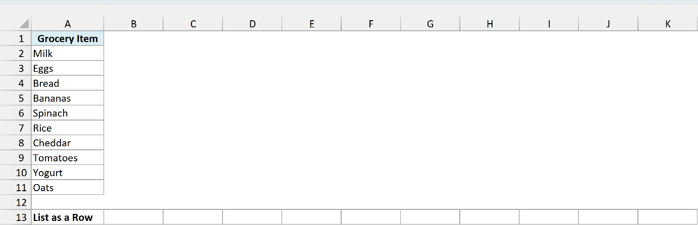
Here is the formula:

=TRANSPOSE(A2:A11)

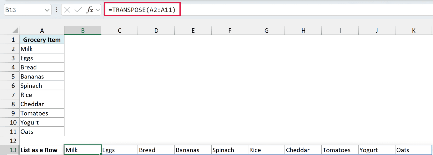
The ten items spill into B13:K13: Milk, Eggs, Bread, Bananas, Spinach, Rice, Cheddar, Tomatoes, Yogurt, and Oats.

The TRANSPOSE function reads the ten cells stacked in the column and returns them side by side. The order stays the same, so top to bottom becomes left to right.

It works the other way too. Give it a row and it returns a column, as you’ll see in Example 4.

If anything blocks the result cells or the output cannot fit on the sheet, Excel returns a #SPILL! error.

Clear anything blocking the result cells and check that the whole output fits on the sheet.

A spilling formula also can’t sit inside an Excel Table. Enter it outside the table, with enough empty cells for the result.

Example 2: Transpose a Whole Table

Now let’s rotate an entire table, headers and all.

Below I have a coffee shop price list, and I want drinks across the top and sizes down the side to compare prices by size, starting in column F.

Here is the formula:

=TRANSPOSE(A1:D5)

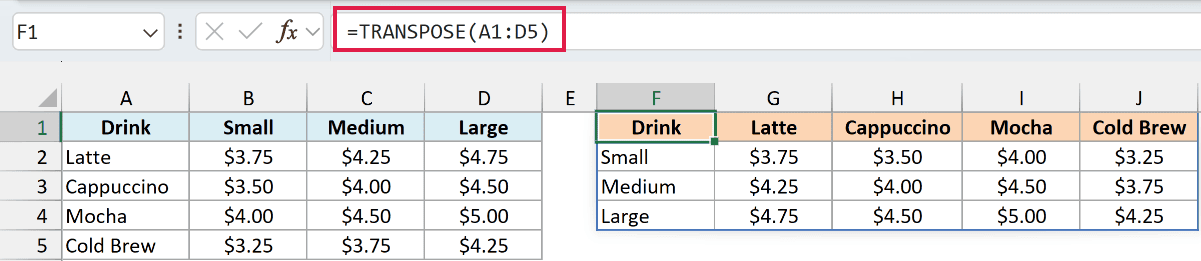
The source is 5 rows by 4 columns, so the result spills into F1:J4 as a block that is 4 rows by 5 columns.

F1:J1 now reads Drink, Latte, Cappuccino, Mocha, and Cold Brew. Small, Medium, and Large run down the first column below Drink.

The corner label in A1 moves with the block, so ‘Drink’ now sits in F1 above the size names, which aren’t drinks.

Because the source range includes the headers, both sets of labels move with the prices.

The Medium Mocha price, $4.50, lands where the Mocha column meets the Medium row.

Pro Tip: The TRANSPOSE function brings values and formula results, not formatting. Apply currency formats, fills, and borders to the result yourself.

Date formats and column widths stay behind too. In the example file, G2:J4 already has the currency format, which is why the prices display with dollar signs.

Example 3: Keep Blanks From Becoming Zeros

Here’s a quirk that trips people up, along with the fix.

Below I have a week of workout minutes, and I want each day’s minutes in column B, with the days in column A.

Wed and Sat are rest days, so their minutes cells are empty. The other values are 45, 30, 50, 35, and 60, in day order.

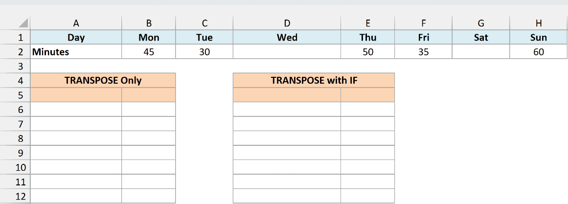
Here is the formula:

=TRANSPOSE(A1:H2)

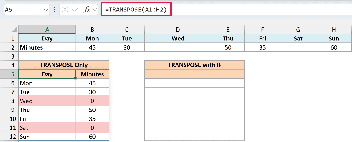
The result fills A5:B12, including the Day and Minutes headers. But notice that Wed and Sat come back as 0 instead of staying blank.

Those zeros read like logged 0-minute workouts. They would also drag down the result of the AVERAGE function.

That’s because zeros count in the average while empty cells don’t.

To keep the blanks blank, wrap the source in the IF function before flipping it. Enter this version in D5.

Here is the formula:

=TRANSPOSE(IF(A1:H2="","",A1:H2))

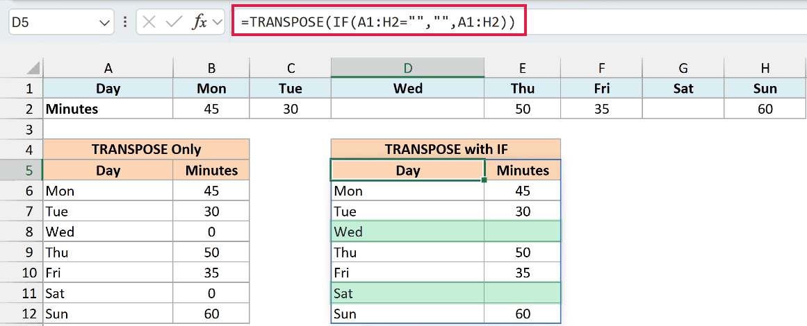
Now D5:E12 shows the same week, with the minutes beside Wed and Sat left blank.

Here is how this formula works:

• The IF function checks every cell in A1:H2 with A1:H2="".
• When a cell is empty, IF returns "", an empty text string that looks blank.
• Otherwise, IF passes the original value through unchanged. A workout time such as 45 stays a real number.
• TRANSPOSE flips the array that IF returns, turning the two source rows into two columns.

You may also see =TRANSPOSE(A1:H2&"") used to keep blanks blank. That turns every number into text too, so 45 becomes “45”.

Use the version with the IF function when you want to keep the workout times numeric for calculations.

Example 4: Turn XLOOKUP Results Into a Column

You can also rotate the row returned by a lookup so it fits a report card.

Below I have test scores for ten students in five subjects, and I want the scores for the student named in H2 in column I.

H2 holds Saoirse, whose scores will appear beside the subject names.

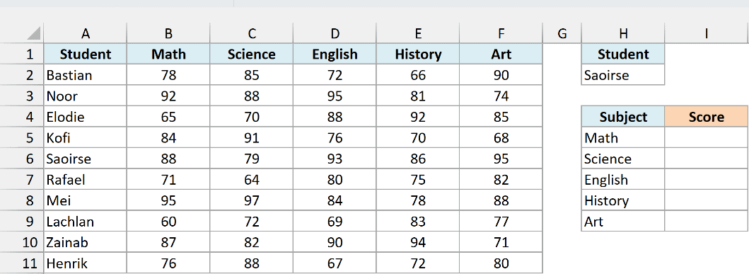
Here is the formula:

=TRANSPOSE(XLOOKUP(H2,A2:A11,B2:F11))

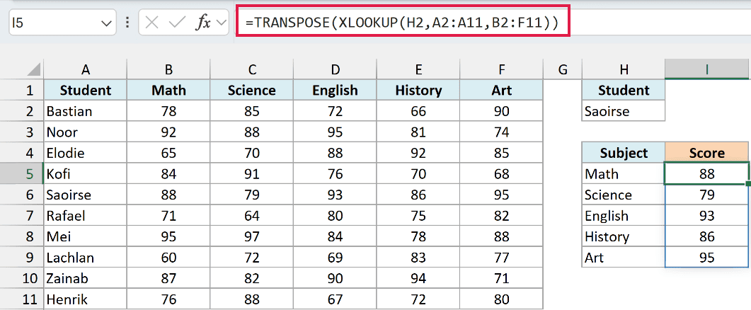
The scores spill into I5:I9: 88, 79, 93, 86, and 95, matching Math, Science, English, History, and Art.

Here is how this formula works:

• The XLOOKUP function finds Saoirse, the name in H2, in A2:A11.
• It returns her whole score row from B2:F11. That gives five values side by side.
• TRANSPOSE stands that row up into a column so the scores line up with the subject list in H5:H9.

Type a different name, such as Mei, in H2 and the report card updates automatically.

This example needs Excel 365 or Excel 2021 and later because it uses the XLOOKUP function.

Example 5: Lay Filtered Names Across a Row

Now let’s pull out only the names you need and turn that list sideways.

Below I have a guest list with party sizes and Yes or No RSVPs, and I want the Yes guests across row 13 for a name-tag strip, starting in column B.

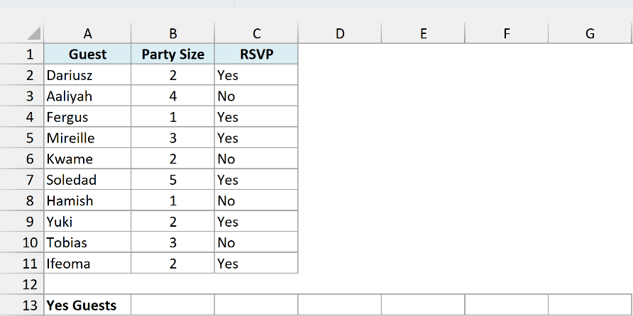
Here is the formula:

=TRANSPOSE(FILTER(A2:A11,C2:C11="Yes"))

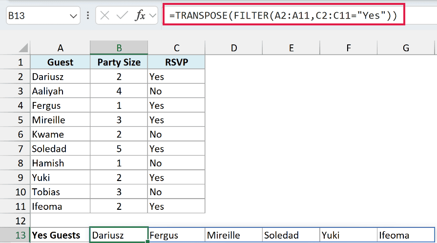
Six guests replied Yes, so B13:G13 fills with Dariusz, Fergus, Mireille, Soledad, Yuki, and Ifeoma.

Here is how this formula works:

• The FILTER function checks C2:C11 for “Yes” and pulls the matching names from A2:A11 as a vertical list.
• TRANSPOSE turns that vertical list into a horizontal row, keeping the names in their source order.

Both functions stay live. Change Kwame’s RSVP to Yes and his name joins the row automatically. The result grows by one cell, so keep the next cell clear too.

This example needs Excel 365 or Excel 2021 and later because it uses the FILTER function.

Example 6: Build Summary Headers and Totals

Let’s finish by using a list of categories to build a summary across the sheet.

Below I have an expense log with twelve entries, and I want each category listed once across row 1, starting in column F.

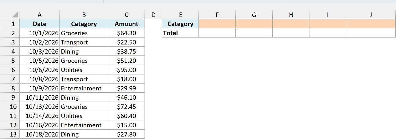
Here is the formula:

=TRANSPOSE(UNIQUE(B2:B13))

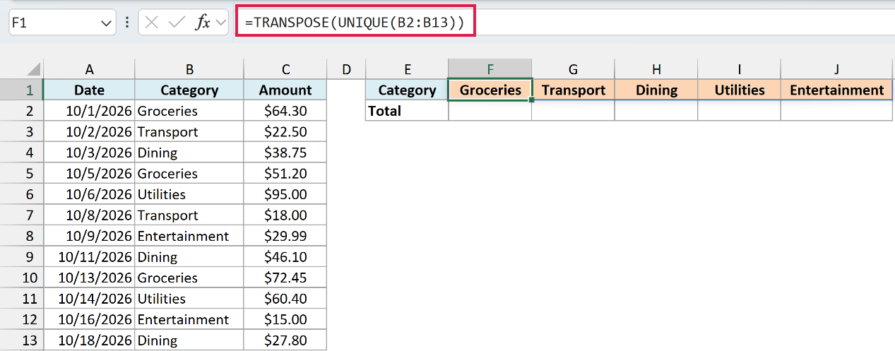
F1:J1 fills with Groceries, Transport, Dining, Utilities, and Entertainment, in the order they first appear in the log.

Here is how this formula works:

• The UNIQUE function returns the five distinct categories in B2:B13 as a vertical list.
• TRANSPOSE turns that list into a horizontal row of category headers.

Now let’s total the expenses for each header with a formula in F2.

Here is the formula:

=SUMIFS(C2:C13,B2:B13,F1#)

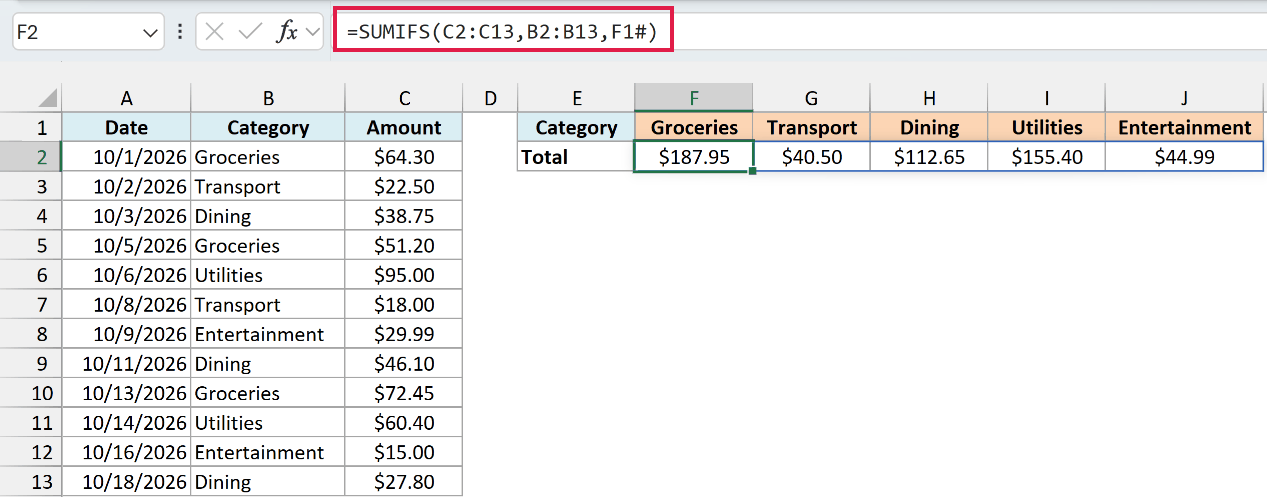
F2:J2 shows $187.95, $40.50, $112.65, $155.40, and $44.99, in the same category order as the headers above.

Here is how this formula works:

• The SUMIFS function adds the amounts in C2:C13 where the categories in B2:B13 match a header.
• F1# is a spill reference. It means the whole spilled range that starts in F1, so it gives SUMIFS all five category headers.
• SUMIFS returns one total per header, spilling all five totals across the row from F2.

If a new category appears within B2:B13, the header row and totals both grow by a column on their own. Keep enough empty space to the right.

These formulas use fixed source ranges. If you add entries below row 13, expand the source ranges in both formulas to include them.

This summary needs Excel 365 or Excel 2021 and later for the UNIQUE function and spilling results.

Pro Tip: For A to Z headers, use =TRANSPOSE(SORT(UNIQUE(B2:B13))) in F1. The SUMIFS formula needs no change.

I’ve shown you how to flip a list or table and rotate another formula’s results to fit your layout.

I hope you found this article helpful.

List of All Excel Functions

Other Excel Articles You May Also Like:

• Convert Columns to Rows in Excel
• How to Flip Data in Excel
• Transpose Multiple Rows into One Column
• GROUPBY Function in Excel
• SORT Function in Excel
• Lookup the Second, the Third, or the Nth Value in Excel
• 20 Advanced Excel Functions and Formulas (for Excel Pros)