

If your text has stray spaces before it, after it, or doubled up between words, the TRIM function is the quickest way to clean it up.
It removes leading and trailing spaces and squeezes any run of spaces between words down to a single space.
This is the kind of mess you get all the time from copied or imported data, and TRIM handles it in one short formula. In Excel 365, you can also feed TRIM a whole range and the cleaned results will spill into the cells below.
In this article, I’ll show you how to use TRIM with practical examples, from a basic cleanup to fixing broken lookups, counting words when the spacing is a mess, and the one type of space TRIM can’t remove on its own.
Follow along with the example file
TRIM Function Examples.xlsx
TRIM Syntax
Here is the syntax of the TRIM function:
=TRIM(text)
- text – the text you want to remove the extra spaces from. This can be a piece of text in quotes, a cell reference, or a range of cells.
TRIM has just one argument, and it’s required. It removes every leading and trailing space, and reduces multiple spaces between words to a single space.
TRIM works in every version of Excel, including Microsoft 365, Excel 2024, 2021, 2019, 2016, and older, plus Excel on the web.
When to Use TRIM in Excel
Use the TRIM function when you need to:
- Clean up text that has extra spaces at the start, the end, or between words
- Fix data pasted or imported from websites, PDFs, or other systems
- Stop lookups and comparisons from failing because of invisible trailing spaces
- Prepare messy text before joining, matching, or counting it
Let me show you a few practical examples of how TRIM works.
Example 1: Remove Extra Spaces From a List of Text
Let’s start with a simple cleanup.
Below is a list of product names that were exported from an inventory system. Some have spaces in front, some have trailing spaces, and a few have double or triple spaces between words.
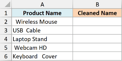
I want a clean version of this list with all the extra spaces stripped out.
Here is the formula:
=TRIM(A2:A6)
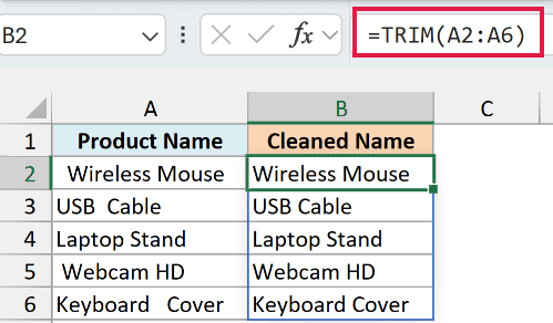
In Excel 365, this one formula in cell B2 spills the cleaned results down the whole range. Each product name loses its leading and trailing spaces, and the doubled-up spaces between words collapse to one.
Pro Tip: On Excel 2019 or earlier, write the formula for the first cell as =TRIM(A2) and copy it down the column. There’s no spilling in those versions, so you fill it down the old way.
Example 2: Fix a Lookup That Fails Because of Extra Spaces
Here’s a problem that drives people crazy, and TRIM is usually the fix.
Below I have a small reference table with employee IDs in column A and their department in column B. In cell B7, I’ve pasted an employee ID that came from a web form, and it has an invisible trailing space after it.
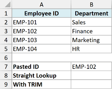
I want to look up the department for the ID in B7.
Here is the straight lookup:
=XLOOKUP(B7,A2:A5,B2:B5)
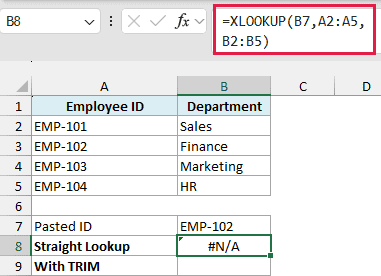
This returns #N/A. To Excel, “EMP-102 ” with a trailing space is not the same text as “EMP-102” in the table, so it finds no match. Extra spaces like this are one of the sneakiest reasons for formulas not working the way you expect.
Now let me wrap the lookup value in TRIM:
=XLOOKUP(TRIM(B7),A2:A5,B2:B5)
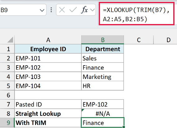
This returns Finance. TRIM strips the trailing space off B7 before the lookup runs, so the value now matches “EMP-102” in the table exactly.
Pro Tip: On Excel 2019 or earlier where XLOOKUP isn’t available, use the same trick with VLOOKUP: =VLOOKUP(TRIM(B7),A2:B5,2,FALSE). If the extra spaces are in the lookup table instead of the search value, clean the table with TRIM first.
Example 3: Clean Imported Data With TRIM and CLEAN
Now let’s look at messier data.
Below is a column of support notes that were copied out of a web app. Along with extra spaces, the cells contain line breaks in the middle of the text, which leaves the entries broken across lines.
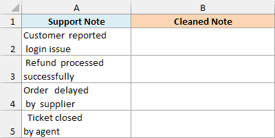
I want each note cleaned up into a single tidy line.
Here is the formula:
=TRIM(CLEAN(A2:A5))
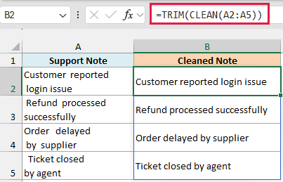
TRIM on its own only deals with spaces, so it can’t remove those line breaks. Here CLEAN runs first and strips out the line breaks and other non-printing characters, then TRIM tidies up the spaces that are left behind.
The result is each note on one clean line, with single spaces between words.
These notes have spaces beside the line breaks. CLEAN deletes the breaks, so words can join together if no space separates them.
Example 4: Remove Non-Breaking Spaces That TRIM Misses
This next one trips up a lot of people, so it’s worth knowing.
Below is a list of city names copied from a web page. They look like they just have leading spaces, but TRIM won’t clean them. That’s because the “space” is actually a non-breaking space, the character web pages use, which has a code of 160.
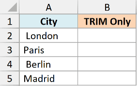
I want these names cleaned up with the leading space gone.
Here is TRIM on its own:
=TRIM(A2:A5)
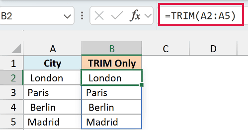
The values come back looking exactly the same. TRIM only removes the regular space character (code 32), so the non-breaking space (code 160) survives.
The fix is to swap that non-breaking space for a normal space first, using SUBSTITUTE, and then let TRIM do its job:
=TRIM(SUBSTITUTE(A2:A5,CHAR(160)," "))
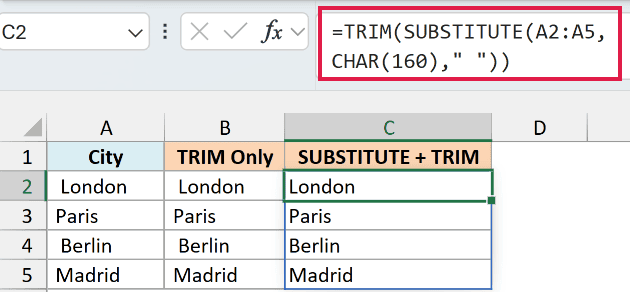
Now the names come back clean. SUBSTITUTE turns every non-breaking space (CHAR(160)) into a regular space, and TRIM removes it along with any other extra spaces.
Example 5: Fix Numbers Stored as Text With Leading Spaces
Extra spaces don’t just make text look messy. They can also stop numbers from adding up.
Below are invoice amounts that were imported as text. Each one has a leading space, so Excel treats them as text, not numbers, and a SUM on the column returns 0.
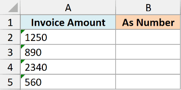
I want these turned into real numbers I can add up.
Here is the formula:
=VALUE(TRIM(A2:A5))
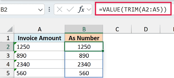
TRIM removes the leading spaces, but it still returns text. VALUE then converts that cleaned text into an actual number, so the results can be summed, averaged, or used in any calculation.
Pro Tip: If VALUE still throws a #VALUE! error after TRIM, the leading character is probably a non-breaking space, not a regular one. Wrap the reference in SUBSTITUTE(A2,CHAR(160),” “) first, like in Example 4, then apply TRIM and VALUE.
Example 6: Count Words Correctly When There Are Extra Spaces
Here’s a handy one that catches a lot of people out.
Below are a few short feedback comments pulled from a survey. Some have double spaces between words, and a couple have leading or trailing spaces.
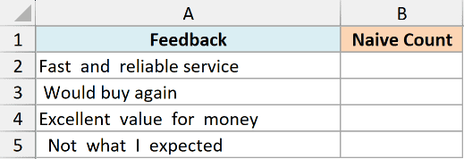
I want an accurate word count for each comment, no matter how messy the spacing is.
The usual way to count words is to count the spaces and add 1:
=LEN(A2:A5)-LEN(SUBSTITUTE(A2:A5," ",""))+1
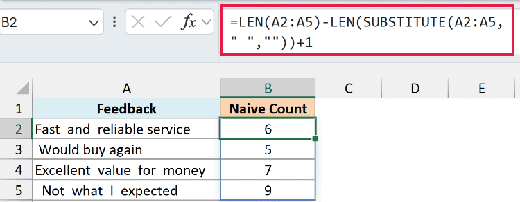
SUBSTITUTE strips every space out, so the difference in length is the number of spaces. Add 1 and you get the word count.
But look at the results. The counts come back too high, because every extra space gets counted as if it were another gap between words.
Wrapping the text in TRIM first fixes it:
=LEN(TRIM(A2:A5))-LEN(SUBSTITUTE(A2:A5," ",""))+1
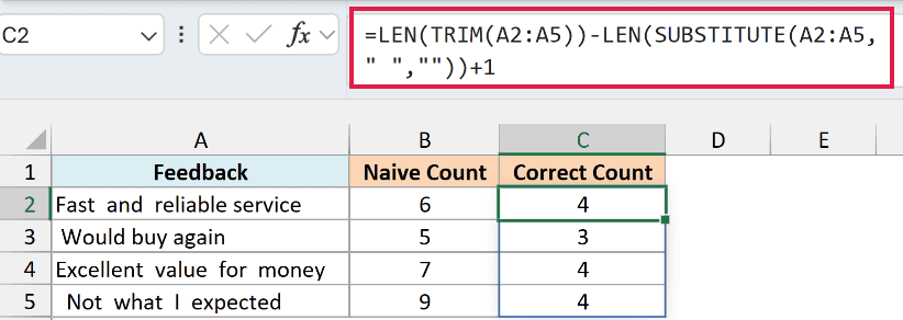
TRIM collapses the double spaces and drops the leading and trailing ones, so LEN(TRIM(…)) counts only the real single spaces between words. Each nonempty comment now returns its true word count. Blank cells and cells containing only spaces return 1 with this formula.
Pro Tip: In Excel 365 you can also count words with =COLUMNS(TEXTSPLIT(TRIM(A2),” “)). TEXTSPLIT breaks the trimmed text into separate words and COLUMNS counts them.
Example 7: Remove Only the Leading Spaces
Sometimes you don’t want TRIM to touch everything.
Below is a list of addresses. The parts of each address are separated by double spaces on purpose to make them easier to read, but a few rows also picked up accidental spaces at the start.
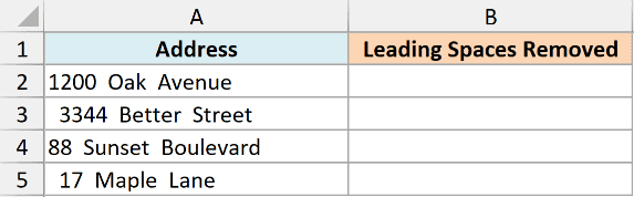
I want to strip only the leading spaces and keep the intentional double spacing between the address parts.
Plain TRIM won’t work here, because it would also collapse the double spaces I want to keep. Here is a formula that removes just the leading spaces:
=RIGHT(A2:A5,LEN(A2:A5)-FIND(LEFT(TRIM(A2:A5),1),A2:A5)+1)
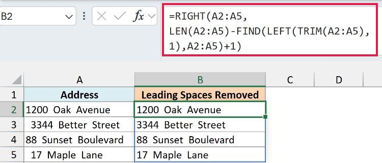
How this formula works:
- LEFT(TRIM(A2:A5),1) grabs the first real character of each address, ignoring any leading spaces. For ” 3344 Better Street” it returns “3”.
- FIND(…) locates where that first character sits in the original text. Here “3” is in the third position, since two leading spaces come before it.
- LEN(A2:A5) minus that position, plus 1 gives the length of the address once the leading spaces are gone.
- RIGHT(…) then pulls that many characters from the right. That returns everything after the leading spaces while leaving the double spaces between words intact.
You can adapt the same idea to strip only trailing spaces, or only leading and trailing spaces, by changing which side you measure from.
Tips & Common Mistakes
- TRIM does not remove every space. It only trims the regular space character (code 32). Non-breaking spaces (code 160) from web content survive, so pair TRIM with SUBSTITUTE when data comes from a website.
- TRIM keeps single spaces between words. It won’t strip out all spaces. If you need to remove every space, including the ones between words, use SUBSTITUTE(A1,” “,””) instead.
- TRIM returns text. Even when the cleaned value looks like a number, it’s still text. Wrap it in VALUE to get a real number you can calculate with.
- Replace the original messy data. TRIM leaves your source column untouched. Once the cleaned results look right, copy them and use Paste Special > Values over the original column, then delete the helper formulas.
- Reach for CLEAN for the invisible stuff. TRIM handles spaces, but line breaks and other non-printing characters need CLEAN. Combine them as TRIM(CLEAN(A1)) for a thorough cleanup, and see these other ways to clean data in Excel.
TRIM is one of those small functions you end up using constantly once you work with data from other people or other systems.
Whether you’re cleaning a list, fixing a broken lookup, or getting imported numbers to add up, it’s usually the first thing to try.
Just remember its one blind spot, the non-breaking space, and keep SUBSTITUTE handy for when TRIM alone isn’t enough.
Other Excel Articles You May Also Like:
