

If you have a formula that sometimes returns an error like #N/A or #DIV/0!, and you want to show something friendlier in its place, the IFERROR function is what you need.
It checks your formula, and the moment it hits an error, it swaps in a value you choose.
In Excel 365, you can also hand IFERROR a whole range and it cleans up every error in one spilled formula.
In this article, I’ll show you how to use IFERROR with real examples, from catching division errors to handling failed lookups and adding up a column that contains errors.
Follow along with the example file
IFERROR Function Examples.xlsx
IFERROR Syntax
Here is the syntax of the IFERROR function:
=IFERROR(value, value_if_error)
- value – the formula or expression you want to check for an error. This is usually a calculation or another function like a lookup.
- value_if_error – what to return when value evaluates to an error. It can be text, a number, a blank (
""), or even another formula.
Both arguments are required. If value doesn’t return an error, IFERROR just hands back its normal result.
Pro Tip: IFERROR catches every error type Excel throws, including #N/A, #VALUE!, #REF!, #DIV/0!, #NUM!, #NAME?, and #NULL!. If you only want to catch a failed lookup (#N/A) and still see the rest, use IFNA instead. More on that later in this article.
IFERROR works in Excel for Microsoft 365, Excel 2024, 2021, 2019, 2016, and Excel on the web.
When to Use IFERROR
Use the IFERROR function when you want to:
- Replace an ugly error value with a clean message or a blank cell in a report.
- Handle a lookup that comes up empty, so you show “Not found” instead of #N/A.
- Avoid a #DIV/0! error when a denominator might be zero or blank.
- Add up a column that has a few error cells in it without the total breaking.
Let me show you a few practical examples of how this works.
Example 1: Catch a Division Error with IFERROR
Let’s start with one of the most common cases: division that sometimes breaks.
Below is a table of ad campaigns, with the campaign name in column A, the number of conversions in column B, and the ad spend in column C. A couple of campaigns had zero conversions.
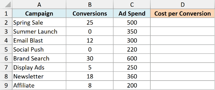
I want the cost per conversion for each campaign, without a #DIV/0! showing up for the campaigns that had no conversions.
Here is the formula:
=IFERROR(C2:C9/B2:B9,"No conversions")
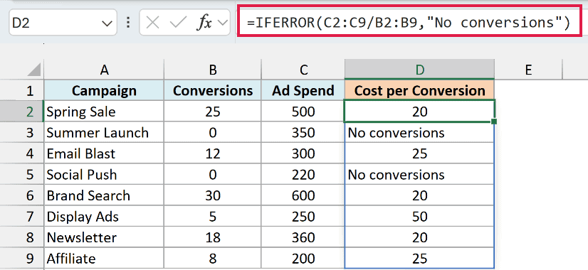
Here C2:C9/B2:B9 divides the spend by the conversions for every row at once. When a campaign has zero conversions, that division returns a #DIV/0! error, and IFERROR replaces it with the text “No conversions”.
Because I passed whole ranges, the formula spills a result down the column on its own. You type it once and Excel fills the rest. No dragging.
Pro Tip: The spilling version works in Microsoft 365, Excel 2021, Excel 2024, and Excel for the web. On Excel 2019 or earlier, put =IFERROR(C2/B2,”No conversions”) in the first cell and copy it down.
If you want to understand what causes it in the first place, here is how to get rid of the #DIV/0! error in Excel.
Example 2: Show a Message When a Lookup Fails
A classic use of IFERROR is cleaning up a lookup that doesn’t find a match.
Below I have an employee list, with the employee ID in column A and the department in column B. In cell D2 I can type an ID to look up.
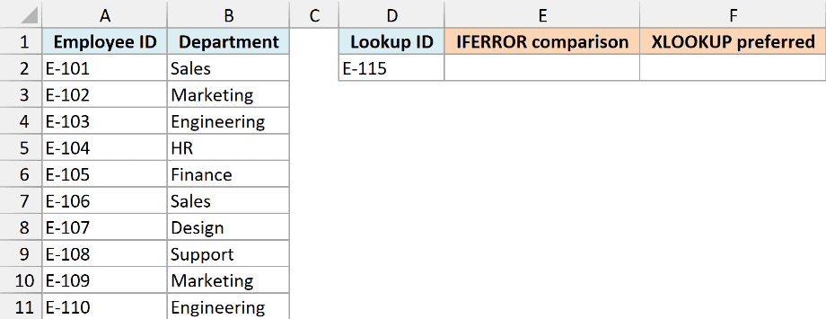
I want to type an employee ID in D2 and get their department back, but show a clear message when the ID isn’t in the list.
Here is the formula:
=IFERROR(XLOOKUP(D2,A2:A11,B2:B11),"ID not found")
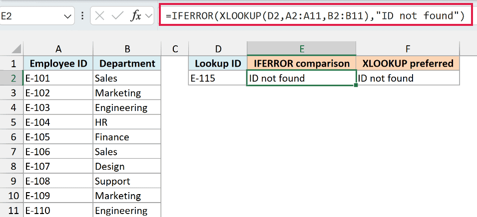
The XLOOKUP function looks for the ID from D2 in column A and returns the matching department from column B. When the ID isn’t there, XLOOKUP returns #N/A, and IFERROR turns that into “ID not found”.
Pro Tip: XLOOKUP has its own if_not_found argument: =XLOOKUP(D2,A2:A11,B2:B11,”ID not found”). Use that for missing IDs. Unlike IFERROR, it leaves an error in a matched department cell visible. XLOOKUP works in Microsoft 365, Excel 2021, Excel 2024, and the web.
For VLOOKUP, IFNA handles #N/A and IFERROR handles broader errors. Here is how to wrap VLOOKUP in IFERROR to get rid of #N/A errors.
Example 3: Flag Text Where a Word Isn’t Found
IFERROR is also handy with functions that error when they don’t find something, like SEARCH.
Below I have a list of customer comments in column A. I want to check which ones mention the word “refund”.
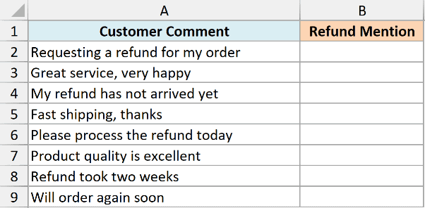
I want the position where “refund” appears in each comment, and the text “Not mentioned” when the word isn’t in that comment.
Here is the formula:
=IFERROR(SEARCH("refund",A2:A9),"Not mentioned")
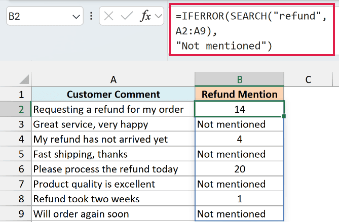
SEARCH returns the position where “refund” starts in the comment. When the word isn’t there, SEARCH returns a #VALUE! error, and IFERROR swaps in “Not mentioned” instead.
This spills down the whole column from a single formula. SEARCH also ignores case, so it finds “Refund” and “refund” alike.
Pro Tip: A #VALUE! error can pop up for a few different reasons. If you keep running into one, here is how to fix the #VALUE! error in Excel.
Example 4: Sum a Column That Contains Errors
Here’s one that saves a lot of headaches. If a column has even one error cell, a plain SUM returns an error too. IFERROR lets you add up the good values and ignore the bad ones.
Below I have a payout table, with the region in column A and the payout in column B. A few payout cells still show #N/A from a lookup that didn’t find a match.
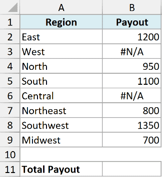
I want the total payout across all regions, even though some cells contain #N/A and a normal SUM would just return #N/A as well.
Here is the formula:
=SUM(IFERROR(B2:B9,0))
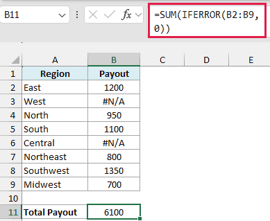
IFERROR runs across the whole range B2:B9 and turns every error into a 0. SUM then adds up the cleaned-up array, so the errors count as nothing and you get a real total.
This example shows how IFERROR works inside another formula. If you only need the sum, AGGREGATE can ignore error values directly. The reader file includes that comparison in Example 4.
In Microsoft 365 and Excel 2021 you just press Enter. There is no need for the old array-formula key combo here.
Pro Tip: On Excel 2019 or earlier, enter this one with Ctrl + Shift + Enter so it works as an array formula. In 365 and 2021, a plain Enter is all you need.
IFERROR vs IFNA: Which Should You Use?
Since these two look similar, it’s worth knowing when to reach for each.
IFERROR catches every error type. That’s convenient, but it can hide a real problem. If your own formula has a bug, like a #REF! from a deleted column, IFERROR quietly shows your fallback text and you never spot the mistake.
IFNA catches only #N/A. That includes a missing match and a #N/A already present in a matched result cell. Other errors still show through for you to fix.
Here is the same lookup from Example 2, written with the employee ID in column A and the department in column B, this time with IFNA.
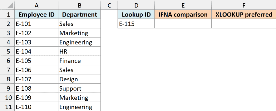
I want the same “ID not found” message for a missing ID, but I still want to see any other error if the formula itself breaks.
Here is the formula:
=IFNA(XLOOKUP(D2,A2:A11,B2:B11),"ID not found")
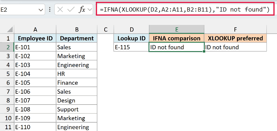
This behaves just like the IFERROR version for a missing ID. The difference shows up when another error occurs, since IFNA leaves errors other than #N/A visible.
If you only want to handle a missing ID, use XLOOKUP’s own if_not_found argument. It preserves an error in a matched department cell, including #N/A.
As a rule of thumb, use IFNA for lookups where you only expect a not-found situation, and use IFERROR when you genuinely want to swallow any error.
Tips & Common Mistakes
A few things to keep in mind when you use IFERROR:
- It hides every error, including your bugs. IFERROR masks #REF!, #NAME?, and the rest along with the one you meant to catch. Wrap the smallest piece that can fail, not the whole formula, so a real mistake still surfaces.
- A blank-looking result is text, not truly empty. Using
""as the fallback leaves an empty string. COUNTBLANK counts it, but ISBLANK returns FALSE because the cell still contains a formula. - value_if_error can be another formula. You can point it at a second lookup, so if the first source fails, IFERROR tries the next one. That’s how people chain fallback sources into one formula.
- Don’t use it to paper over a fixable error. If a #REF! means a column got deleted, fix the reference instead of hiding it. IFERROR is for expected errors, not broken formulas.
- It’s been around a long time. IFERROR was added in Excel 2007. Before that people combined the IF function with ISERROR, which you don’t need anymore.
Wrapping Up
IFERROR is one of those small functions that makes your spreadsheets a lot cleaner. Catch a division error, handle a lookup that comes up empty, or add up a column with a few bad cells, and the messy error values disappear.
Just remember to wrap only the part that can fail, so a real mistake still gets your attention. I hope you found this tutorial helpful.
Other Excel Articles You May Also Like:
