

If you have a formula that suddenly shows #NUM! instead of a result, it means Excel ran into a number it cannot work with. This happens when a calculation produces an invalid numeric value or a result that falls outside the range Excel can handle.
The good news is that #NUM! almost always points to one of the specific causes, so it is easy to fix once you know what to look for.
In this article, I’ll walk you through the common reasons you see the #NUM! error and show you exactly how to fix each one.
What the #NUM! Error Actually Means
Before we jump into the fixes, it helps to know what Excel is telling you.
The #NUM! error shows up when a formula or function gets a number it cannot use. Maybe the value is too big, maybe it is mathematically impossible, or maybe a function ran out of attempts trying to find an answer.
So #NUM! is not a typo error or a missing-reference error. It is specifically about numbers that Excel cannot process. Each cause below has its own fix, so let’s go through them one by one.
Cause 1: The Number Is Too Large or Too Small for Excel
Let’s start with the most basic one.
The biggest number you can type into a cell is about 9.99999999999999E+307. A calculation can go a little higher, up to about 1.797E+308, but push a result past that and you get the #NUM! error.
A simple way to trigger this is to raise 10 to a huge power.
=10^1000
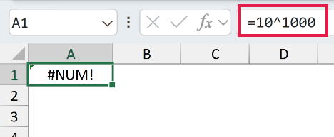
This returns #NUM! because 10 to the power of 1000 is far larger than Excel’s maximum number.
You will also see this with factorials. The FACT function works fine up to FACT(170), but the moment you go one higher, the result blows past Excel’s limit.
=FACT(171)
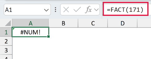
This also returns #NUM!, since FACT(171) is bigger than the largest number Excel can store.
The same thing happens in the other direction. Excel’s limit is about -1.797E+308, so a result far below zero overflows just as easily.
=-9E+307-9E+307
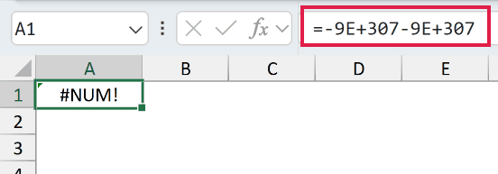
Each number here is perfectly valid on its own. It is the total, roughly -1.8E+308, that lands just outside Excel’s range, so you get #NUM!.
Pro Tip: “Too small” here means far below zero, not close to zero. A tiny fraction is not a #NUM! problem at all. Excel simply rounds it off, so =10^-1000 returns 0 rather than an error.
How do you fix this?
There is no way to make Excel store a number it cannot hold, so the fix is to rework the calculation.
If you only need a relative comparison, work with the logarithm of the values instead of the raw numbers. That keeps the figures small enough to handle.
If the giant number came from a mistake (like an exponent that should have been much smaller), correct the input so the result lands inside Excel’s range.
Cause 2: A Function Got an Invalid Argument
Some functions only accept certain values. Give them something outside that range and they return #NUM!.
The classic example is taking the square root of a negative number. There is no real square root of a negative value, so SQRT gives up.
=SQRT(-9)
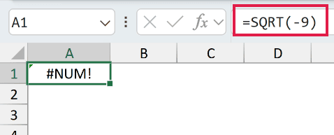
This returns #NUM! because -9 is negative.
How do you fix this?
If the value should have been positive in the first place, fix the source data. But if you genuinely want the square root of the absolute value, wrap the number in ABS first.
=SQRT(ABS(-9))
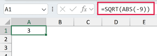
ABS converts -9 into 9, so SQRT now returns 3.
The same idea applies to LOG and similar functions. LOG only works on positive numbers, so feeding it zero or a negative value returns #NUM! too. Check that the number going in is positive before the function runs.
LARGE and SMALL break the same way, just with a different rule. You tell them which position you want, and if that position does not exist in your range, there is nothing for them to return.
Here I have five sales figures in A2:A6, and I have asked LARGE for the eighth largest value.
=LARGE(A2:A6,8)
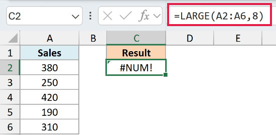
This returns #NUM! because there are only five numbers in the range. There is no eighth largest value to give back. Asking for position 0 or a negative position does the same thing.
The fix is to ask for a position that actually sits inside the range. With five values, any position from 1 to 5 works.
=LARGE(A2:A6,3)
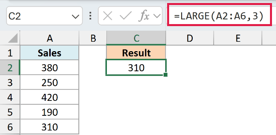
Now the formula returns 310, which is the third largest number in the list.
Cause 3: IRR Needs Both a Negative and a Positive Value
Now let’s look at the financial functions, because they trip people up in two different ways. This is the first one.
IRR works out the return on a series of cash flows. For it to have anything to solve, those cash flows have to include both money going out and money coming in.
Microsoft puts it plainly: the values must contain at least one positive value and one negative value. A common slip is to point IRR at just the return rows and leave the initial investment out.
Below is the dataset. It’s a simple bond. B2 holds the -1000 you put in, B3:B6 hold the 120 interest you collect each year, and B7 holds the final 1120, which is your 1000 back plus the last 120 of interest.
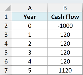
Here is the formula that causes the problem:
=IRR(B3:B7)
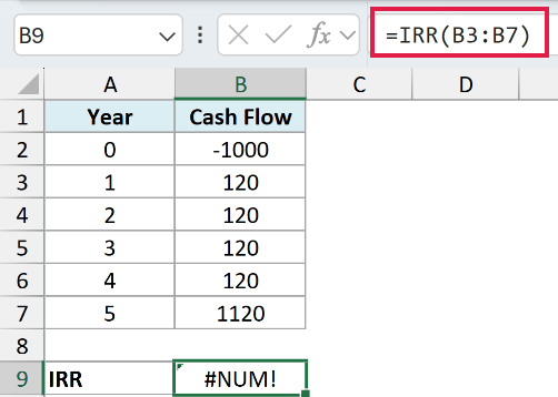
This returns #NUM!. The range B3:B7 covers only the positive returns and skips the outflow in B2, so every number is positive and there is no rate to solve for.
How do you fix this?
Include the initial outflow in the range so IRR has both a negative and a positive value to work with.
=IRR(B2:B7)
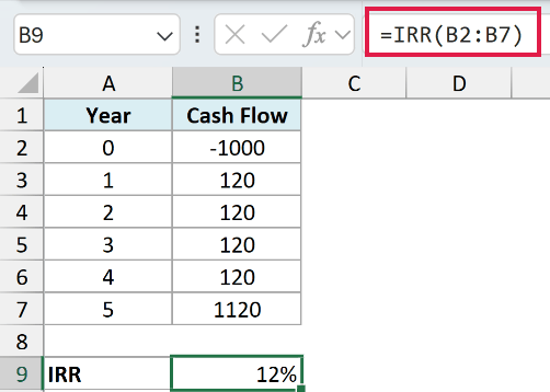
Now the range runs from the -1000 in B2 through the returns. IRR has money going out and coming back, so it settles on a valid rate of 12 percent.
Cause 4: IRR or RATE Cannot Settle on an Answer
Here is the second way the financial functions bite, and it looks identical from the outside.
IRR and RATE do not work out their answer directly. They start from a guess and keep refining it until the number stops moving.
That refining has a limit. Both functions give up after 20 tries, and if they have not landed on an answer by then, they hand you #NUM!.
The starting guess is usually what decides it. Leave the guess out and both functions assume 10 percent, which can be nowhere near the real answer.
Say you borrowed 1000 and agreed to pay back 3000 per period for two periods. That is a brutal rate, and RATE cannot get to it from the default guess.
=RATE(2,-3000,1000)
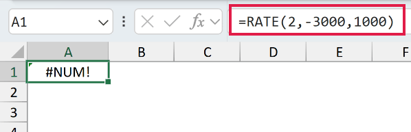
This returns #NUM!. The real rate is a long way from the 10 percent RATE starts at, so it runs out of tries before it ever gets close.
How do you fix this?
Give the function a starting guess nearer the answer. Guess is the last argument of RATE, and the second argument of IRR.
=RATE(2,-3000,1000,0,0,0.5)
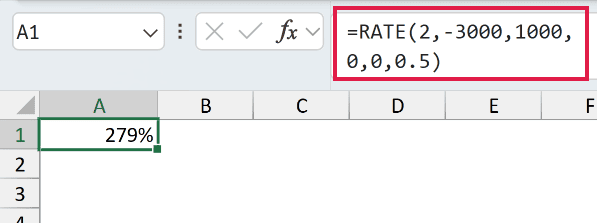
Starting from 0.5 instead of 10 percent, RATE gets there and returns 279 percent. Microsoft notes that RATE usually converges when the guess is between 0 and 1.
A guess only helps when there is a rate to find, though. If the cash flows are all one sign, like in Cause 3, no guess will rescue them, so check the signs first.
Pro Tip: You may run into advice to fix this with File > Options > Formulas > Enable iterative calculation. That setting only governs circular references. IRR and RATE run their own fixed 20-try limit, so changing it does nothing here. The guess argument is the lever that actually works.
Cause 5: The Start Date Is Later Than the End Date
This one trips up a lot of people using DATEDIF.
DATEDIF expects the start date first and the end date second. If you accidentally put the later date first, Excel cannot count backwards, so it returns #NUM!.
Let’s say you want the number of days between 1 January 2023 and 1 January 2024, but you entered the dates in the wrong order.
=DATEDIF("1-Jan-2024","1-Jan-2023","d")
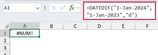
This returns #NUM! because the start date is later than the end date.
How do you fix this?
Swap the dates so the earlier one comes first.
=DATEDIF("1-Jan-2023","1-Jan-2024","d")
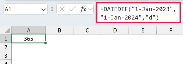
Now the dates are in the right order, and the formula returns 365.
If your dates live in cells, just make sure the start-date cell holds the earlier date and the end-date cell holds the later one.
How to Hide a #NUM! Error With IFERROR
This last one is not a cause. It is what you do once you know a #NUM! can show up and you would rather not stare at it.
Sometimes you cannot avoid an occasional #NUM!, and you just want a cleaner message instead of the raw error showing up in your sheet.
For that, you can wrap your formula in IFERROR. It checks the result, and if it is an error, it shows your custom text instead.
=IFERROR(SQRT(A2),"Check input")
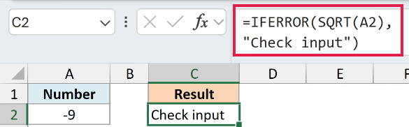
If A2 holds a valid number, you get the square root. If A2 is negative and SQRT throws #NUM!, the cell shows “Check input” instead.
One important caveat. IFERROR hides the error, it does not fix it. The underlying problem (in this case, a negative input) is still there.
It is also not fussy about which error it catches. A #REF! or a #VALUE! in that same formula would show “Check input” too, which can bury a completely different problem.
So use IFERROR to tidy up the display, not as a substitute for tracking down the real cause.
Things to Keep in Mind
- #NUM! is always about numbers, not references or text. If you are seeing #REF! or #VALUE! instead, those have different causes, so make sure you are actually dealing with a #NUM! before applying these fixes.
- Check the function’s argument rules first. Most #NUM! errors come from feeding a function a value it does not accept, like a negative number into SQRT or LOG, or a position that does not exist into LARGE, so reading what the function expects usually points you straight to the fix.
- For IRR, XIRR, and RATE, the guess argument is your friend. If the function errors out, try a few different starting guesses, and double-check that your cash flows include both positive and negative values.
- IFERROR is a display tool, not a repair tool. It is great for keeping a report clean, but always confirm the underlying formula is actually correct before you wrap an error away.
In this article, I showed you what the #NUM! error means and how to fix each of its common causes, from oversized numbers and bad arguments to date order and iterative functions like IRR and RATE.
I hope you found this article helpful.
Other Excel Articles You May Also Like:
