IRR Function in Excel

If you want to know what rate of return a project or an investment is actually earning you, the IRR function in Excel is what you’re looking for. You give it the cash flows, and it hands back the internal rate of return.

IRR returns a single value, but it works fine inside dynamic array formulas, so one =BYCOL(...) formula can give you the IRR of several projects at once.

In this tutorial, I’ll show you how to calculate IRR in Excel, how it’s different from NPV, and what to do when your cash flows don’t arrive at neat intervals.

This Tutorial Covers:

What Is IRR (Internal Rate of Return)?

IRR is a discount rate that is used to measure the return of an investment based on periodical incomes.

The IRR is shown as a percentage, and you can use it to decide whether a project is profitable for a company or not.

Let me explain IRR with a simple example.

Suppose you’re planning to buy a company for $50,000 that will generate $10,000 every year for the next 10 years. You can use this data to calculate the IRR of this project, which is the rate of return you get on your $50,000.

In this example, the IRR comes out to be about 15%. That means it’s equivalent to investing your money at a 15% rate of return for 10 years.

Once you have the IRR value, you can use it to make decisions. If you have another project where the IRR is more than 15%, you should invest in that one instead.

Or if you’re planning to take a loan and buy this project for $50,000, make sure the cost of the capital is less than 15%. Otherwise you pay more for the capital than you make from the project.

IRR Syntax

Excel lets you calculate the internal rate of return using the IRR function. Here is the syntax:

=IRR(values, [guess])

values – a reference to the cells (or an array) that hold the cash flows you want the internal rate of return for. This one is required.
guess – a number you think is close to the IRR. It’s optional, and Excel uses 0.1 (10%) when you leave it out. IRR works out the answer by trying rates over and over, so the guess is just where it starts looking.

Here are some important prerequisites for using the function:

The cash flows must contain at least one negative and one positive value. The negative one is usually your initial investment.
IRR only looks at numbers. Text, logical values, and empty cells are ignored, not treated as zero.
The guess must be a percentage entered as a decimal (if you provide it at all).
The cell holding the result should be formatted as a percentage.
The amounts must arrive at regular intervals (months, quarters, years).
All amounts must be in chronological order, because IRR reads the order of the values as the order of the cash flows.

Pro Tip: If your cash flows come in at different time intervals, use the XIRR function instead, which lets you specify a date for every cash flow. I’ve covered this in Example 6 below.

When to Use IRR

Use the IRR function when you need to:

Work out the rate of return on a project from its cash flows.
Check a project’s return against your cost of capital before you commit to it.
Rank a few competing projects and see which one earns the most.
Find the point at which an investment starts paying for itself.
Convert a series of messy, uneven incomes into one number you can compare.

Now let’s have a look at some examples to better understand how to use the IRR function in Excel.

Example 1: Calculate IRR for a Series of Cash Flows

Let’s start with a simple example.

Below is the dataset where a business spent $30,000 on rooftop solar panels in year 0, and then column B shows what it saved on electricity in each of the next six years. The initial spend is negative because the money went out.

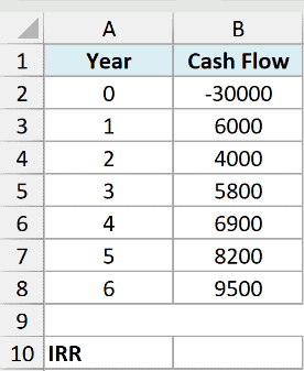
A dataset in Excel showing a $30,000 investment in year 0 followed by six years of cash inflows.

I want the internal rate of return on this $30,000 over the full six years.

Here is the formula:

=IRR(B2:B8)

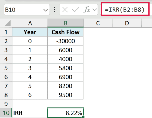
The IRR function in Excel returning an internal rate of return of 8.22% for the series of cash flows.

The result is 8.22%, which is the IRR of this cash flow after six years.

In the above formula, IRR reads the whole range as one series of cash flows, in the order the cells sit in the column. It then finds the single rate at which those savings are worth exactly the $30,000 you paid up front.

Notice the range starts at B2, the negative $30,000. Leave that cell out and IRR has nothing to earn a return on, so it returns a #NUM! error.

Example 2: Find Out When the Investment Turns Positive

Here’s another practical scenario.

You can also calculate the IRR for every period in a cash flow and see when exactly the investment starts to have a positive internal rate of return.

Let’s stick with the same rooftop solar dataset from Example 1, with the $30,000 spend in year 0 and the six years of savings in column B.

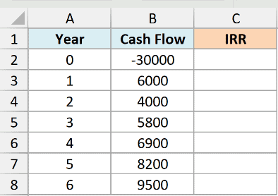
The same cash flow dataset with an empty IRR column ready to hold the running internal rate of return for each year.

I want to know the year in which the IRR of this investment turns positive, which tells me when the project breaks even.

To do this, instead of calculating the IRR for the entire project, we work out the IRR as of each year. Here is the formula in cell C3, which you then copy down the column:

=IRR($B$2:B3)

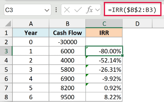
The IRR function with a mixed cell reference copied down the column, showing the internal rate of return as of each year and when it first turns positive.

As you can see, the IRR after year 1 is -80.00%, after year 2 it’s -52.14%, and after year 3 it’s -26.31%.

It’s still negative in year 4, crosses zero in year 5 at 0.92%, and finishes at 8.22%, the same answer Example 1 gave us.

So this investment has a positive IRR after the fifth year. Before that, you haven’t made your $30,000 back yet.

Note that the reference in the above formula is a mixed cell reference. The first reference ($B$2) is locked with dollar signs before the column letter and the row number, and the second one (B3) is not.

That way, when you copy the formula down, it always starts at the initial investment and stretches to the row the formula sits in.

Pro Tip: This is handy when you have to choose between two projects with a similar IRR. The one whose IRR turns positive faster is usually the safer bet, since you get your capital back sooner.

Example 3: Compare Multiple Projects with IRR

Now let’s look at something a bit more useful.

The IRR function can also be used to compare several projects and see which one is the most profitable.

Below is a dataset for three projects. Row 2 holds the initial investment in each one (shown as a negative, since it’s money going out), and the rows under it hold six years of cash flow from each.

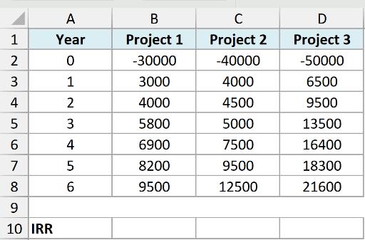
A dataset in Excel comparing the cash flows of three projects, each with its initial investment in row 2.

I want the IRR of each project so I can see which one earns the most.

Here is the formula for Project 1:

=IRR(B2:B8)

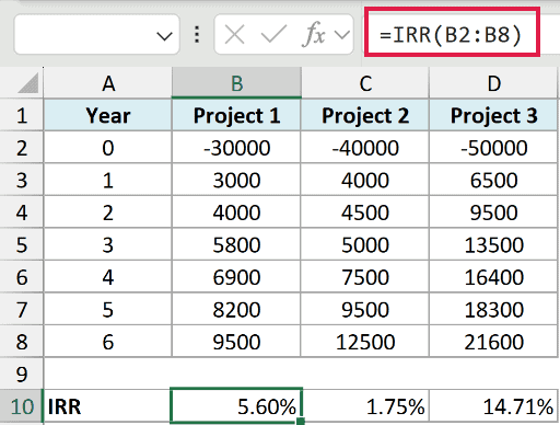
The IRR function calculating the internal rate of return for each of the three projects, showing 5.60%, 1.75%, and 14.71%.

Copy it across and you get the other two as well. Project 1 comes out at 5.60%, Project 2 at 1.75%, and Project 3 at 14.71%.

If we suppose the cost of capital is 4.50%, Project 2 is not acceptable, since it earns less than the money costs. Project 3 clears the bar comfortably, and Project 1 clears it but not by much.

Since IRR takes an array, you can also get all three in one formula instead of copying anything across:

=BYCOL(B2:D8, LAMBDA(cash_flows, IRR(cash_flows)))

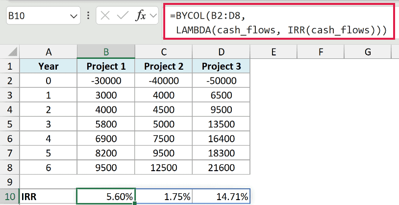
A single BYCOL formula calculating the internal rate of return of all three projects at once and spilling the results across.

BYCOL hands each column of the range to IRR one at a time, and the three results spill across three cells. This needs Excel 365 or Excel 2024.

Definition: If you’re wondering what a cost of capital is, it’s what you pay to get access to the money. Take $100K as a loan at 4.5% a year and your cost of capital is 4.5%. And if you issue preferential shares promising a 5% return to raise $100K, your cost of capital would be 5%. Most companies raise money from several places at once, so their cost of capital is a weighted average of all of those sources.

So if you have to make a decision to invest in only one project, go with Project 3. And if you could invest in more than one, invest in Project 1 and 3.

One thing to watch here. IRR is a rate and not an amount, so it won’t tell you which project puts the most money in the bank. There’s more on this in the IRR vs NPV section below.

Example 4: When a Project Has More Than One IRR

Let’s step it up with something most people never run into until it bites them.

Below is a dataset for a small gravel quarry. It costs $160,000 to open in year 0, sells $1,000,000 of gravel in year 1, and then the lease requires $1,000,000 of land restoration in year 2.

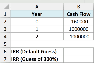
A dataset for a gravel quarry showing a cost in year 0, a large inflow in year 1, and a large cleanup cost in year 2.

I want the internal rate of return on this quarry.

Here is the formula:

=IRR(B2:B4)

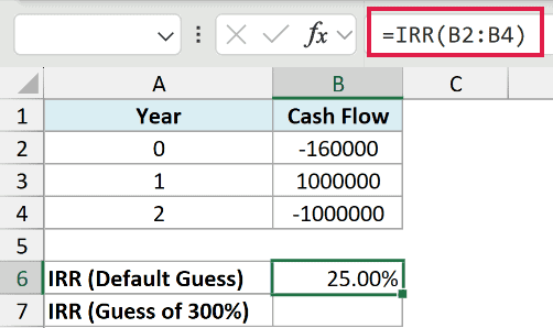
The IRR function returning 25.00% for a cash flow series that changes sign twice.

This returns 25.00%. Looks great. But watch what happens when I nudge the guess up to 300%:

=IRR(B2:B4,3)

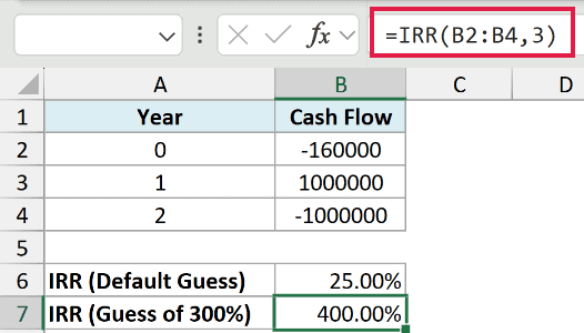
The same IRR function with the guess argument raised to 300%, now returning 400.00% for the same cash flows.

Same cash flows, and now the answer is 400.00%. Both are genuinely correct, and this quarry actually has two IRRs.

What happens is that the cash flow changes sign twice here (out, in, then out again). Once that happens, a project can have more than one IRR, and Excel just returns whichever one it lands on from the guess you gave it.

Now add the three cash flows up. The quarry loses $160,000 overall. Two healthy-looking IRRs, and the project still isn’t worth doing.

Note: The guess argument is not there to make IRR more accurate. It only tells Excel where to start looking. Change it and you can land on a different (but equally valid) IRR, exactly like above.

Example 5: Calculate an Annual IRR from Monthly Cash Flows

Here’s one that trips people up constantly.

Below is a dataset for a vending machine route that cost $18,000 to buy, with the cash it generated in each of the next twelve months.

A dataset for a vending machine route showing the purchase cost and the cash it generated in each of the next twelve months.

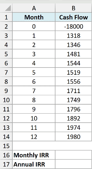
I want the annual rate of return on this route, not the monthly one.

Let’s do the plain IRR first:

=IRR(B2:B14)

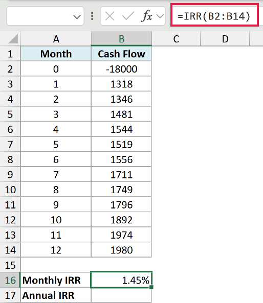
The IRR function returning a monthly internal rate of return of 1.45% for the monthly cash flows.

That gives 1.45%, and it’s easy to read it as a terrible investment. It isn’t. IRR gives back a rate for whatever period your cash flows use, and these are monthly, so 1.45% is a monthly return.

To get the annual figure, compound it over twelve months:

=(1+IRR(B2:B14))^12-1

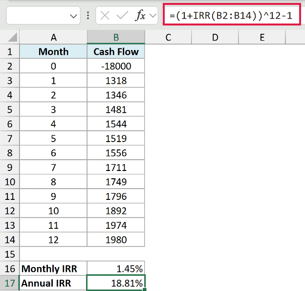
The monthly internal rate of return compounded over twelve months to give an annual figure of 18.81%.

Now you get 18.81% a year, which is a very different story.

You’ll see people multiply the monthly rate by 12 instead, which gives 17.36% here. That’s the nominal rate, and it quietly ignores the fact that each month’s cash can be put back to work.

Pro Tip: If your cash flows are irregular rather than monthly, don’t bother with this at all. XIRR (Example 6) already returns an annualized rate.

Example 6: Calculate IRR for Irregular Cash Flows (XIRR)

Now let’s tackle the biggest limitation of the IRR function.

IRR assumes your cash flows are periodic, with the same gap between every one of them. In real life, projects pay off whenever they feel like it.

Below is a dataset for an investment where the cash flows land at completely irregular intervals. The dates are in column A and the amounts are in column B.

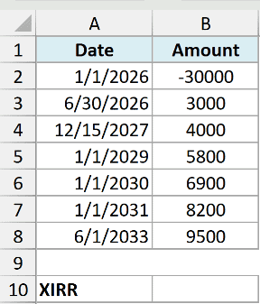
A dataset in Excel where the cash flows land on irregular dates rather than at even yearly intervals.

I want the rate of return on this $30,000, taking the actual dates into account.

Here, we can’t use the regular IRR function, but there’s another function that can do this, the XIRR function. XIRR takes the cash flows as well as the dates, which lets it account for the uneven gaps.

Here is the formula:

=XIRR(B2:B8,A2:A8)

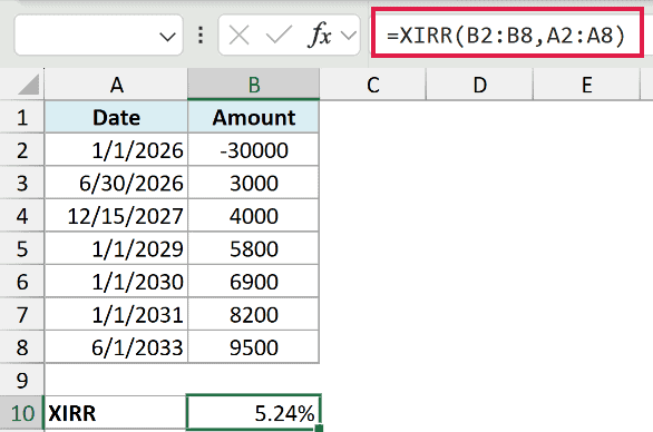
The XIRR function returning an internal rate of return of 5.24% for cash flows that land on irregular dates.

The result is 5.24%. In the above formula, the cash flows are the first argument and the dates are the second.

XIRR treats the first date in the list as day zero and discounts everything after it using a 365-day year. So the number it gives you is always an annual rate, whatever the gaps look like.

Note: If XIRR returns a #NUM! error, add a third argument with a rough guess of the return you expect. It doesn’t have to be exact or even close. It just gives the formula a better place to start from.

Example 7: Calculate IRR in Excel Without the IRR Function

Let’s finish with a way to get the IRR without touching the IRR function at all.

This is worth knowing for two reasons. It shows you what IRR is really doing under the hood, and it’s a nice sanity check when a result looks off.

Below is the same rooftop solar dataset from Example 1, with four extra cells set up. D2 and D3 hold the labels, E2 holds a starting rate of 10%, and E3 will hold the net present value at that rate.

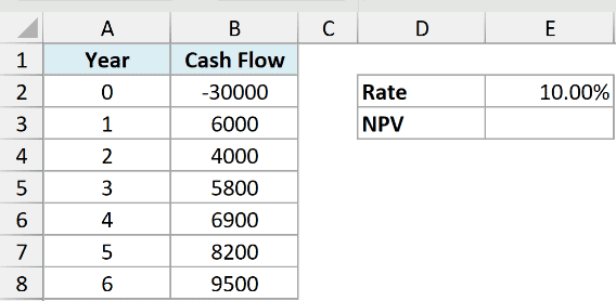
The rooftop solar cash flows with a rate cell and an NPV cell set up next to them, ready for Goal Seek.

I want to find the rate that makes the net present value of these cash flows come out to exactly zero, because that rate is the IRR.

Here is the formula in E3:

=NPV(E2,B3:B8)+B2

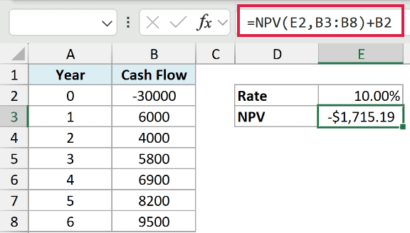
An NPV formula with the initial investment added back outside the function, returning a negative net present value at a 10% rate.

Notice that the $30,000 in B2 sits outside the NPV function. That’s because Excel’s NPV discounts its first cash flow by one full period, and your year 0 spend happens today, so it shouldn’t be discounted at all.

Now go to Data > What-If Analysis > Goal Seek.

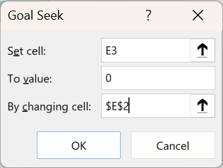
The Goal Seek dialog box in Excel set to drive the NPV cell to zero by changing the rate cell.

Set cell E3 To value 0 By changing cell E2, then hit OK.

Goal Seek walks the rate up and down until the NPV hits zero, and lands on roughly 8.22%, the same answer =IRR(B2:B8) gave us in Example 1.

Goal Seek stops as soon as it’s close enough, so the last decimal or two can drift a little from what IRR returns. It’ll be near enough to confirm the number.

IRR vs NPV – Which Should You Use?

When it comes to evaluating projects, both NPV and IRR are used, but NPV is the more reliable method.

NPV is the Net Present Value method, where you discount all the future cash flows and see what they’re worth in today’s money. If that value is higher than your initial outflow, the project is profitable.

IRR answers a different question. It tells you the rate at which you’d have to discount all those future cash flows to end up with exactly what you paid today.

So if you spend $100K on a project with an IRR of 10%, discounting every future cash flow at 10% gets you back to $100K.

Both are used when evaluating projects, and sometimes they disagree with each other. When they do, go with the NPV recommendation.

IRR has a few drawbacks that make NPV the safer call:

The reinvestment assumption. The IRR math implicitly assumes every cash flow the project throws off gets reinvested at the same IRR. That’s usually unrealistic, since most of that money ends up in other projects or in something safe like bonds, earning far less. (Excel’s MIRR function exists to fix exactly this.)
Multiple IRRs. When the cash flows flip sign more than once, the project can have more than one IRR, as you saw in Example 4. Excel doesn’t warn you. It just shows whichever one it converged to.
It ignores size. IRR is a rate, so a tiny project can out-score a much bigger one that would make you far more money. A $10K project earning 20% beats a $1M project earning 12% on rate alone, while the bigger one makes you far more.

Despite its shortcomings, IRR is a good way to evaluate a project, and it works well alongside NPV when you’re deciding which projects to pick.

Tips & Common Mistakes

Blank cells aren’t zeros. IRR skips empty cells entirely rather than reading them as zero, which quietly shifts every later cash flow one period earlier and changes your answer. Type a 0 into any period with no cash flow.
You need one negative and one positive number. With all-positive values, there’s no investment to earn a return on and IRR returns #NUM!.
A #NUM! error is usually a convergence problem, not a bug. Excel tries up to 20 times to land within 0.00001% of the answer. If it can’t, you get #NUM!. Feeding it a guess closer to the real answer often gets it there.
Format the result cell as a percentage. Otherwise 8.22% shows up as 0.082247, and it looks like something broke.
Keep your cash flows in chronological order. IRR reads the order of the cells as the order of the periods. Sort the range and you’ll get a different, wrong answer.
Rows must be evenly spaced in time. Yearly, quarterly, monthly, whatever you like, but the same gap throughout. Uneven gaps mean XIRR, not IRR.
The rate matches your period. Monthly cash flows give a monthly IRR. Compound it as shown in Example 5 before you compare it to anything annual.
If your cash flows are all equal, RATE is quicker. RATE is built for level payments, so you don’t need a column of repeated numbers just to feed IRR.

In this tutorial, I showed you how to use the IRR function in Excel, from a simple cash flow all the way to comparing projects and spotting a project with two IRRs.

I also covered how to calculate the IRR for irregular cash flows using the XIRR function, and how to get the same number without the IRR function at all using Goal Seek.

I hope you found this tutorial useful!

List of All Excel Functions

Other Excel Articles You May Also Like: