

If you want to calculate the net present value of a project or an investment in Excel, the NPV function is what you’re looking for. But there is one quirk that trips up almost everybody.
Excel’s NPV function assumes your first cash flow arrives at the end of the first period, not today. Nothing to worry about though, the fix is a small one.
In this article I’ll show you how to calculate NPV in Excel, how to handle that timing quirk, and what to do when your cash flows land on irregular dates.
NPV returns one value for a single discount rate. In dynamic-array Excel, you can pass a range of rates to return one NPV for each rate. I’ll come back to that in Example 6.
Follow along with the example file
NPV Function Examples.xlsx
What is NPV? A Quick Explanation
Before we get into calculating the NPV value, let me quickly explain what it really means.
NPV (short for Net Present Value), as the name suggests, is the net value of all your future cash flows (which could be positive or negative).
For example, suppose there’s an investment opportunity where you need to pay $10,000 now, and you will be paid $1,000 per year for the next 20 years.
If you know the current discount rate (also called the cost of capital or the interest rate), you can use that in the NPV formula in Excel to get the present value of all the future inflows from this investment.
If that value is more than $10,000, the investment has a positive NPV under the assumed cash flows and discount rate. That supports considering it, provided the rate reflects its risk and the project fits your budget and other constraints.
And in case it is less than $10,000, the investment has a negative NPV at that discount rate. Its projected cash flows do not meet that required return, even if it brings in more cash than you originally spent.
The reason this works is simple. A dollar you get five years from now is worth less than a dollar in your hand today, and the discount rate is what puts a number on that gap.
NPV is also used when comparing different projects or investment opportunities.
If you have 3 different projects with expected outflow and inflow values, you can use the net present values of all of these to see which project has the best profitability.
Now that you have a decent understanding of what NPV is, let’s look at the function itself.
NPV Syntax
Excel has an in-built NPV function with the following syntax:
=NPV(rate, value1, [value2], ...)
The above formula takes the following arguments:
- rate – this is the discount rate for one time period. For example, if your cash flows happen every year, this would be the annual discount rate. If these are quarterly, this would be the quarterly discount rate.
- value1 – the first cash flow. This one is required, and it can be positive (inflow/income) or negative (outflow/payment).
- [value2], … – any further cash flows. These are optional, and you can pass up to 254 of these value arguments in total.
Some important things to know when using the NPV function in Excel:
- The NPV function considers all these values to be evenly spaced out (i.e., they have the same time interval between each value).
- The order of the values matters, so if you change the order and keep the same values, the final result would be different.
- The formula considers that the inflow/outflow takes place at the end of each period.
- In arrays and cell references, only numeric values are counted. Blank cells, text, and logical values are ignored.
The most important thing to keep in mind is that you can only use this formula when you have a regular flow of inflows and outflows. If the inflow/outflow happens at the end of the year, it should be the same for all the values.
Pro Tip: In case you have a dataset where the inflow/outflow happens on specific dates (and is not evenly spaced), you can not use the NPV formula. In that case, you need to use the XNPV formula, which I cover in Example 5.
Also read: Calculating Weighted Average in Excel (Using Formulas)
When to Use NPV
Use this function when you need to:
- Work out whether a project or an investment is worth doing at all
- Compare several projects and pick the one that creates the most value
- Put a present-day price on a stream of future payments you have been offered
- Test how much a change in the cost of capital hurts a project’s economics
- Turn a lumpy set of yearly cash flows into one number you can put in front of a decision maker
Let me show you a few practical examples of how to use this function.
Example 1: Calculate NPV in Excel When Cash Flows Start at Year End
Let’s start with a simple example.
Below is the dataset. Column A has the period in years (1 through 6), the cash flows are in B2:B7, and the discount rate of 5% sits in cell D2.
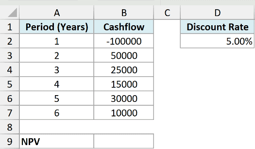
In this example, the first outflow of $100,000 happens at the end of Year 1, and every cash flow after that lands at the end of its own year.
I want the net present value of this whole set of cash flows.
Here is the formula:
=NPV(D2,B2:B7)
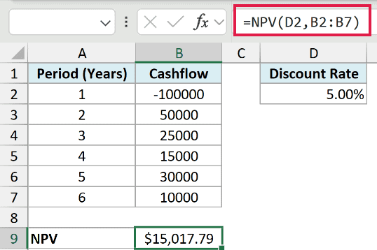
The above formula gives an NPV of $15,017.79. Based on these cash flows and the given discount rate (also called the cost of capital), the project has a positive NPV.
This is the straightforward use of the NPV function. Every value sits at the end of a period, which is exactly what NPV expects, so you can hand it the whole range and be done.
Note that even the $100,000 outflow gets discounted here. NPV divides it by 1.05 because it treats it as money leaving your hands a year from now, not today.
That is fine when the outflow really is a year away. But be careful, because it usually isn’t.
Almost nobody invests a year from now. You pay for it today. So for most real projects, the formula above is not the one you want, and the next example is.
Example 2: Calculate NPV When the Investment Happens Today
Here’s the scenario you’ll actually run into most of the time.
Below I have the same cash flows, laid out a little differently. Column A runs from period 0 to period 5, the cash flows are in B2:B7, and the discount rate of 5% is again in cell D2.
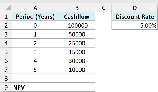
This time the $100,000 goes out today, at the beginning of the first year, and the returns come in at the end of Years 1 through 5.
I want the net present value of this project.
Here is the formula:
=B2+NPV(D2,B3:B7)
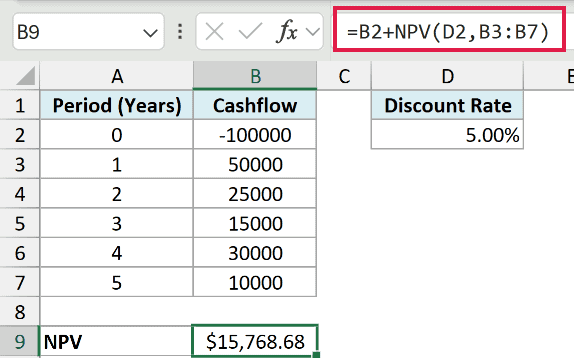
This gives us $15,768.68.
In the above formula, I have left the initial outflow out of the NPV function, because it happens at the beginning of the first year.
The NPV function is built in such a way that it treats every value as an inflow/outflow at the end of a period.
So I excluded the initial outflow, calculated the NPV of the other future cash flows, and then added the outflow back to the result.
Money you spend right now is already in today’s dollars. It doesn’t need discounting, so it has no business being inside the function.
Note that B2 is negative, so +B2 is subtracting the $100,000. You don’t need a minus sign as long as your outflow is entered as a negative number.
So when the first cash flow happens at the beginning of the first period, exclude it from the formula and add it back to the result.
Pro Tip: Putting the entire series, including today’s outflow, inside NPV shifts every cash flow one period later. The result equals the correct NPV divided by 1+rate.
Here, $15,017.79 x 1.05 = $15,768.68. For a negative NPV and positive rate, the wrong result is less negative. A difference by this factor is a clue to check the timing, not proof of the cause.
Example 3: Compare Projects Using NPV to Find the Best One
In real life, it often happens that you need to analyze multiple projects and see which one is best for you or your company.
Below I have three projects side by side. Column A has the period in years (1 through 6), and B2:D7 holds the cash flows for Project 1, Project 2, and Project 3.
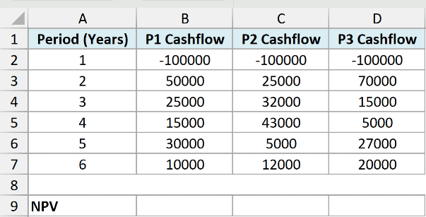
For the purpose of this example:
- I am considering that the first cash flow happens at the end of the first year
- The initial outflow for each project is $100,000
- The discount rate for evaluating all the projects is 5%
I want the net present value of each project, so I can see which one is actually worth doing.
Here is the formula:
=NPV(5%,B2:B7)
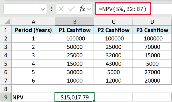
Every cash flow sits at the end of a period here, including the outflow. So the whole column goes inside the function. This is the Example 1 treatment, not the Example 2 one.
That formula sits in B9, under Project 1. Now copy it across to C9 and D9, and it picks up =NPV(5%,C2:C7) and =NPV(5%,D2:D7) on its own. The rate is typed in as a literal 5%, so there is nothing to lock.
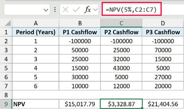
The three numbers:
- Project 1: $15,017.79
- Project 2: $3,328.87
- Project 3: $21,404.56
Based on the results, Project 3 has the highest NPV. If these cash-flow assumptions and the 5% discount rate are appropriate for all three projects, and you can choose only one with no other constraints, it ranks first.
Under the same assumptions, Projects 3 and 1 have the highest combined NPV if you can choose two independent projects and the budget allows both.
Project 2 ranks last here, but its NPV is still positive at $3,328.87. It collects $117,000 against Project 1’s $130,000, and its biggest payday lands in Year 4, so it loses on size and on timing at the same time.
Pro Tip: When evaluating projects using the NPV method, remember that it works on projected future cash flows. With projections, there is always a risk that things don’t turn out as expected (could be higher or lower). The risk of error in forecasting also increases as the duration increases. We can forecast income in the next two years with far more accuracy than income in Year 19 and 20.
Example 4: Calculate NPV for Monthly Cash Flows
Now let’s look at something a bit more interesting.
Below I have a small delivery van purchase. Column A runs from Month 0 to Month 12, the cash flows are in B2:B14, and cell D2 holds the monthly discount rate of 1%.
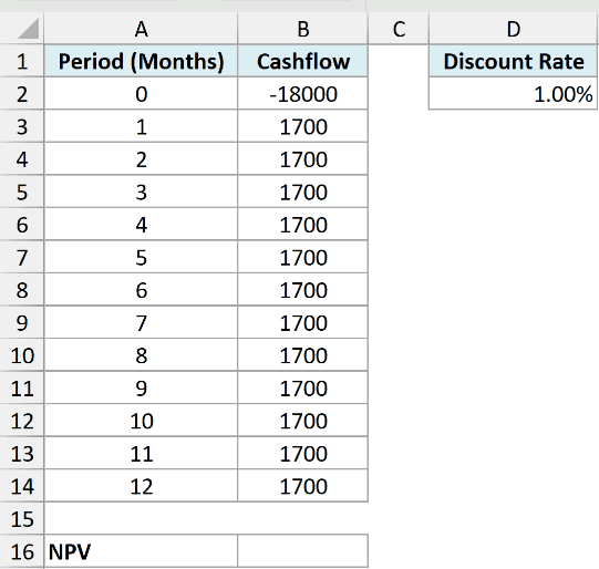
The van costs $18,000 today and is expected to bring in $1,700 at the end of every month for the next 12 months. The example uses a nominal annual cost of capital of 12%, compounded monthly, which works out to 1% a month.
I want to know whether buying the van is worth it.
Here is the formula:
=B2+NPV(D2,B3:B14)
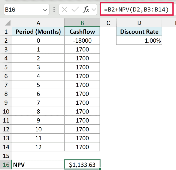
This returns $1,133.63, so the van clears its cost of capital, but not by a lot.
The formula is identical to Example 2. The only thing that changed is the rate.
This is the part people get wrong. Your rate has to match the length of one period in your data. Monthly cash flows need a monthly rate, quarterly cash flows need a quarterly rate.
If you had left 12% in D2 while feeding it monthly cash flows, Excel would have happily charged you 12% of interest per month and told you the van was a terrible idea.
Pro Tip: The conversion depends on how the annual rate is quoted. A nominal annual rate of 12%, compounded monthly, gives 1% a month and an effective annual rate of 12.68%.
For an effective annual rate of 12%, use =(1+12%)^(1/12)-1. This gives 0.9489% a month and an NPV of $1,195.58. Use the conversion that matches your stated annual rate.
Example 5: Calculate NPV for Irregular Intervals Using XNPV
The NPV formula works great if you have regular cash flows (i.e., the time period between the cash flows is the same). But in case it’s not, you can’t use the NPV function.
For such cases, Excel gives you the XNPV function. XNPV is similar to NPV, with one improvement: you can specify a date for each cash flow, and it will work out the present value of each one based on that date.
Below is the syntax of the XNPV formula:
=XNPV(rate, values, dates)
The above formula takes the following arguments:
- rate – the discount rate, always given as an annual rate
- values – the cash flow values, which could be positive (inflow/income) or negative (outflow/payment)
- dates – the dates for each cash flow
Pro Tip: One important thing to remember when using the XNPV formula in Excel is that the first date is treated as the beginning of the time period.
Every other date must be on or after that one, though they don’t have to be in order. XNPV discounts using a 365-day year.
Below is the dataset. The dates of each cash flow are in A2:A7, the amounts are in B2:B7, and the discount rate of 5% sits in cell D2.
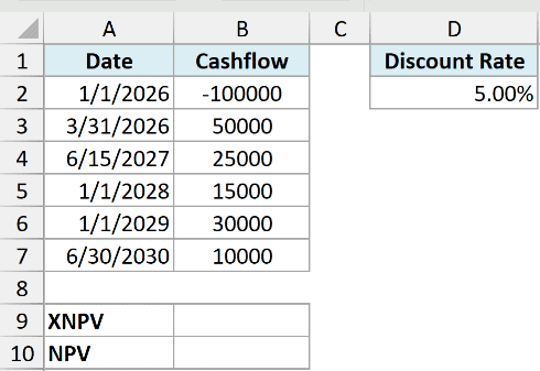
These are the same cash flows as Example 1, with only the dates changed. The $100,000 goes out on January 1, 2026, and the money comes back on five scattered dates through to June 30, 2030. Nothing here is evenly spaced.
I want the net present value of these irregular cash flows.
Here is the formula:
=XNPV(D2,B2:B7,A2:A7)
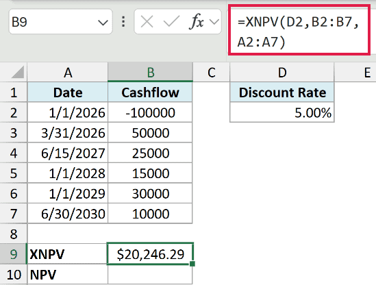
This gives us $20,246.29.
The formula treats the first transaction (the outflow of $100,000 on January 1, 2026) as the starting point, and discounts every later cash flow by the exact number of days between it and that date.
Notice that the initial outflow goes inside XNPV here, not outside it. That’s the opposite of what we did in Example 2, and it’s because XNPV already knows the first date is day zero, so it doesn’t discount it.
It’s worth seeing what NPV makes of the very same data.
To keep this a fair fight, I’m giving NPV its best shot: the Example 2 treatment, with the initial outflow kept outside the function so it isn’t wrongly discounted.
=B2+NPV(D2,B3:B7)
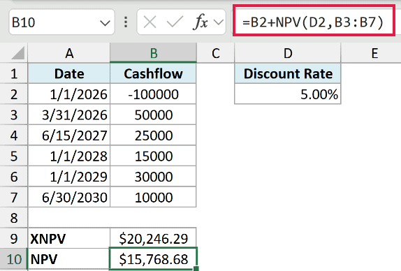
That returns $15,768.68 against XNPV’s $20,246.29, and the NPV answer is wrong. That $15,768.68 should look familiar, because it’s Example 2’s answer. Same money, and NPV can’t see that the timing changed.
The gap is entirely about timing. NPV never looked at column A, so it assumed those five inflows were spaced exactly one year apart.
In reality the first one shows up after 89 days, and the last one after 1,641 days. That’s well short of the five years NPV assumed.
NPV pushed most of that money years further into the future than it really is, and discounted it accordingly. XNPV counted the actual days.
So when you have cash flows happening at irregular time intervals, use XNPV.
Example 6: Check How Sensitive Your NPV Is to the Discount Rate
Let’s step it up with something I use quite often.
Below I have the Example 2 cash flows again, with the $100,000 outflow in B2 and the returns in B3:B7.
Column D holds a list of discount rates from 4% to 8%, and column E is where the NPV of each one will go.
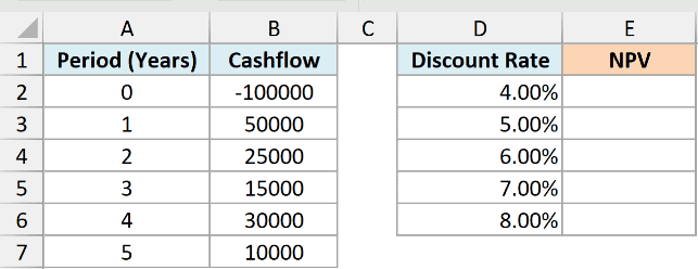
Rather than picking one discount rate and hoping it’s right, I want to see the NPV at every rate in that list at once.
Here is the formula:
=$B$2+NPV(D2:D6,$B$3:$B$7)
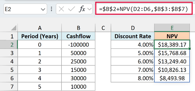
One formula in E2 and the whole column fills itself:
- 4%: $18,389.17
- 5%: $15,768.68
- 6%: $13,249.40
- 7%: $10,826.13
- 8%: $8,493.98
In the above formula, NPV uses each rate in D2:D6 to discount the same future cash flows in B3:B7. Adding B2 includes the $100,000 outflow that happens today.
Passing five rates produces five NPV results, which spill from E2 to E6. The dollar signs keep B2 and B3:B7 fixed, so every rate uses the same cash flows.
The result is worth a look. Move the rate up by four points and the project’s value drops by more than half. A project that looks comfortable at 4% is a lot less comfortable at 8%.
Keep pushing the rate and the NPV eventually hits zero, which for these cash flows happens at about 12%. That number has a name, and it’s the subject of the next section.
Pro Tip: This spilling formula needs Microsoft 365, Excel 2024, Excel 2021, or Excel for the web. On older versions, put =$B$2+NPV(D2,$B$3:$B$7) in E2 and copy it down.
NPV vs IRR: Which One Should You Use?
When analyzing project and investment decisions, NPV and IRR are the two most used methods. Where NPV is Net Present Value and IRR is Internal Rate of Return.
The two are joined at the hip. IRR is simply the rate at which NPV equals zero, which is the 12% we just landed on in Example 6.
Pro Tip: While both methods would give you similar results in most cases, NPV is considered the superior method when it comes to calculating the present value and viability of projects and investments.
IRR has a few shortcomings that make it less reliable, and in some cases the NPV method and the IRR method will give you different results.
Here is where IRR tends to fall down:
- It ignores size. A 40% return on $1,000 beats a 15% return on $1,000,000 on the IRR scale, but the second one makes you far more money.
- It can give more than one answer. If your cash flows flip between positive and negative more than once, there can be several rates where NPV hits zero, and Excel just reports whichever one it finds first.
- It needs a sign change to exist at all. If every cash flow is positive, there’s no rate that drives NPV to zero, and IRR just hands you a #NUM! error. NPV still gives you a number.
NPV doesn’t have these problems. It answers a plainer question: how much value does this add, in today’s dollars?
So in case of different results, the NPV method is considered right. Use IRR to sense-check your answer, but when the two disagree, go with NPV.
Tips & Common Mistakes
- Never leave a gap year blank. Blank cells are ignored, so Excel doesn’t count that year at all and every cash flow after it silently moves one period closer. Type a 0 instead.
- Text and logical values in cash-flow ranges are ignored too. If a cash flow cell holds text that looks like a number, NPV will skip it and shift your timeline, exactly like a blank does.
- The name is a little misleading. If the initial investment happens today, add it outside NPV. If it happens at the end of a period, include it in the cash-flow range. NPV discounts whatever you give it.
- NPV is not PV. PV is for a constant payment repeated over time, like a loan. NPV is for a series of different cash flows. And if you’re working out what that constant payment should be, that’s the PMT function.
- The 254 limit counts arguments, not cells. Listing values one by one caps you at 254. A single range reference like
B2:B7is one argument, so it can hold as many cash flows as you like.
In this tutorial I have covered how to calculate net present value in Excel using the NPV and XNPV functions.
In case you have evenly spaced cash flows, you can use the NPV function. And in case you have irregular cash flows, you can use XNPV (which also uses the dates of the cash flow for the calculation).
Just remember the one rule that catches everybody: if the money goes out today, keep it out of the function and add it back to the result.
I hope you found this tutorial useful!
Other Excel Articles You May Also Like:
