

If you want to work out the payment on a loan, whether it’s a car loan, a mortgage, or a personal loan, the PMT function gives you that number in one formula.
There are two things that trip people up with it. PMT returns a negative payment when the loan amount is positive and the final balance is zero, and the interest rate has to match your payment period.
A monthly payment needs a monthly rate. Both are easy to handle once you know about them.
In Excel 365, you can also feed PMT a range of loan details and it spills a payment for each row, which is handy for comparing offers side by side.
In this article, I’ll show you how to use PMT for loans, mortgages, and savings goals, and how to get the sign and the rate right every time.
Follow along with the example file
PMT Function Examples.xlsx
PMT Function Syntax
Here is the syntax of the PMT function, which calculates the payment for a loan or annuity with a constant interest rate:
=PMT(rate, nper, pv, [fv], [type])
- rate – The interest rate for each period. This is the part people get wrong. If you make monthly payments, the rate must be the monthly rate, so you divide a nominal annual rate by 12 when it is compounded monthly. The examples below use that convention. An effective annual rate needs
=(1+annual_rate)^(1/12)-1instead. - nper – The total number of payments. For a monthly loan this is the number of months, so a 5-year loan is 5*12 = 60.
- pv – The present value, or the loan amount you’re borrowing now (also called the principal).
- fv – (Optional) The balance you want left after the last payment. Leave it out for a normal loan, where the balance ends at 0.
- type – (Optional) When payments are due. Use 0 (or leave it out) for the end of the period, and 1 for the start.
One thing to know up front. With a positive loan amount and a final balance of zero, PMT returns a negative payment to represent money leaving your pocket.
To show it as a positive number, put a minus sign in front of the loan amount, or in front of PMT. I’ll do that in the examples below.
Pro Tip: Keep rate and nper in the same units. Monthly payments need a monthly rate (nominal annual/12) and a count in months (years*12). Mixing an annual rate with a month count is the most common PMT mistake.
PMT works in Excel for Microsoft 365, Excel 2024, 2021, 2019, 2016, and older versions, plus Excel on the web. The spilling range trick in Example 2 needs Microsoft 365, Excel 2024, Excel 2021, or Excel for the web.
When to Use PMT
Use the PMT function when you need to:
- Calculate the monthly payment on a car loan, personal loan, or mortgage
- Compare a few loan offers with different rates or terms at once
- Work out how much to save each month to reach a target amount
- Check how the payment changes when it’s due at the start of the period instead of the end
Let me show you a few practical examples of how PMT works.
Example 1: Calculate a Monthly Loan Payment
Let’s start with a simple car loan.
Below is the dataset. The loan amount is in cell B2, the annual interest rate is in B3, and the loan term in years is in B4.
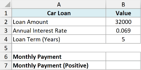
I want the monthly payment on this $32,000 car loan.
Here is the formula:
=PMT(B3/12, B4*12, B2)
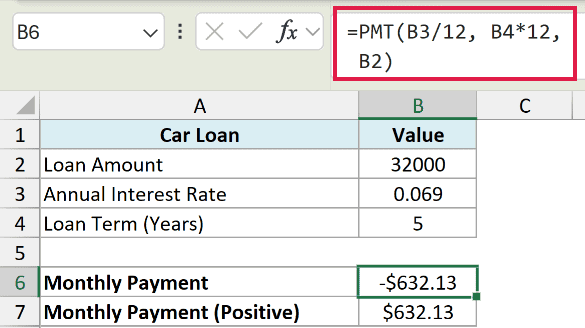
This returns -632.13.
Here, B3/12 turns the 6.9% annual rate into a monthly rate, and B4*12 turns 5 years into 60 monthly payments. The loan amount goes in as the present value.
The result is negative because Excel treats the payment as cash going out. To show it as a positive number, put a minus sign in front of the loan amount.
=PMT(B3/12, B4*12, -B2)
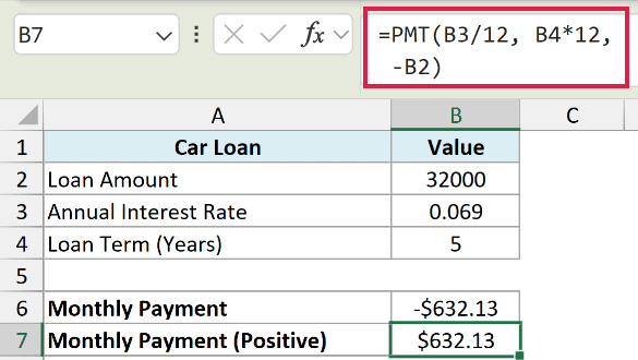
Now the formula returns 632.13, a monthly payment of $632.13.
Example 2: Compare Multiple Loan Offers at Once
Here’s where PMT gets more useful. Say you have three bank offers for the same $28,000 loan, each with a different rate and term, and you want to compare the monthly payments.
Below is the dataset. The bank is in column A, the loan amount in column B, the annual rate in column C, and the term in months in column D.

I want the monthly payment for all three offers in one go.
Here is the formula:
=PMT(C2:C4/12, D2:D4, -B2:B4)
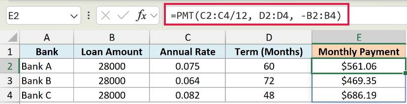
This returns 561.06, 469.35, and 686.19, one payment for each bank.
Because I fed PMT whole ranges instead of single cells, the results spill down the column automatically, one row per offer. You type the formula once in E2 and Excel fills the rest.
The term is already in months here, so only the rate needs dividing by 12. Bank B has the lowest payment, but its 72-month term means you pay for longer.
Example 3: Calculate a Monthly Mortgage Payment
A mortgage works the same way, just with bigger numbers and a longer term.
Below is the dataset. The home loan amount is in B2, the annual interest rate in B3, and the loan term in years in B4.
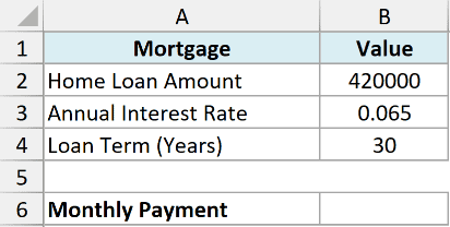
I want the monthly payment on this $420,000 mortgage over 30 years.
Here is the formula:
=PMT(B3/12, B4*12, -B2)
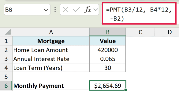
This returns 2654.69, a monthly principal-and-interest payment of $2,654.69. PMT does not include taxes, insurance, reserves, or loan fees.
The 6.5% annual rate is divided by 12, and the 30-year term becomes 360 monthly payments (B4*12). The minus sign in front of B2 keeps the result positive.
Pro Tip: To see the total principal and interest paid, multiply the monthly payment by nper. Here that’s 2654.69 * 360, which is about $955,687 paid over the life of the mortgage. Roughly $535,687 of that is interest.
Example 4: Convert an Annual Rate to a Monthly Rate
This example is about the mistake that catches almost everyone, so it’s worth its own section.
Below is the dataset for a $15,000 personal loan. The amount is in B2, the annual rate in B3, and the term in months in B4.
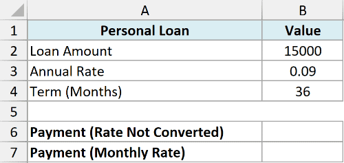
I want to see what happens if I forget to convert the annual rate to a monthly one.
Here is the formula with the annual rate used as-is:
=PMT(B3, B4, -B2)
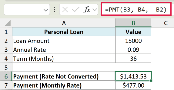
This returns 1413.53, which is way too high. Excel thinks the 9% is a monthly rate, so it’s charging 9% every month.
The fix is to divide this nominal annual rate by 12 so it matches the monthly payments.
=PMT(B3/12, B4, -B2)
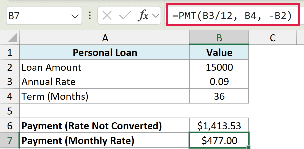
Now the formula returns 477.00, the correct monthly payment of $477.00. The term was already in months, so only the rate needed converting.
Example 5: Work Out Monthly Savings for a Goal
PMT isn’t only for loans. It can also tell you how much to save each month to hit a target, using the fv (future value) argument.
Below is the dataset. The savings goal is in B2, the annual return in B3, and the number of years in B4.
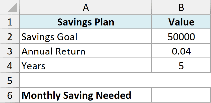
I want to know how much to set aside each month to reach $50,000 in 5 years.
Here is the formula:
=PMT(B3/12, B4*12, 0, -B2)
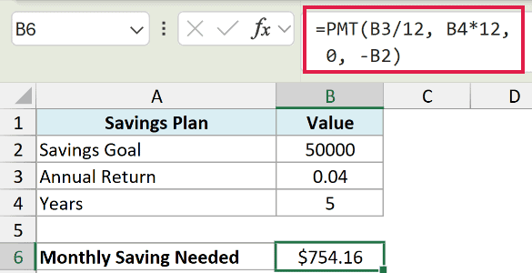
This returns 754.16, so you’d need to save $754.16 a month.
The present value is 0 because you’re starting from nothing, and the goal goes in as the future value. I put the minus sign in front of B2 so the monthly deposit shows as a positive number.
This assumes your savings grow at a steady annual return through compound interest, so it’s an estimate rather than a guarantee.
Example 6: Payments Due at the Start of the Period
By default PMT assumes you pay at the end of each period. The optional type argument lets you switch to the start, which slightly lowers the payment.
Below is the dataset for an $8,000 rent-to-own plan. The amount is in B2, the annual rate in B3, and the term in months in B4.
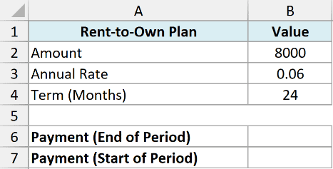
I want to compare the payment when it’s due at the end versus the start of each month.
Here is the formula for payments at the end of the period (the default):
=PMT(B3/12, B4, -B2)
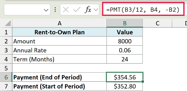
This returns 354.56.
Now here is the same loan with type set to 1, so payments are due at the start of the period.
=PMT(B3/12, B4, -B2, 0, 1)
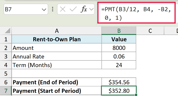
This returns 352.80, a little lower. Paying at the start of the period means each payment reduces the balance a bit sooner, so slightly less interest builds up.
Tips & Common Mistakes
- Match the rate to the payment period. A monthly payment needs a monthly rate (nominal annual/12) and a term in months (years*12). Mixing an annual rate with a month count is the number one PMT error, and it inflates the payment badly, as you saw in Example 4.
- The negative result is normal. With a positive loan amount and a final balance of zero, PMT returns a negative number because the payment is money going out. Put a minus sign in front of the loan amount, or in front of the whole formula, to show it as positive.
- Enter the rate as a rate, not a whole number. Type 6.9% or 0.069, not 6.9. A rate of 6.9 tells Excel you’re paying 690% interest.
- Use IPMT and PPMT for the split. PMT gives the total payment. If you need how much of a specific payment is interest versus principal, use the IPMT and PPMT functions, which take an extra “per” argument for the payment number.
- Feeding ranges spills the results. In Excel 365 and 2021, passing PMT a range for the rate, term, or amount spills a payment for each row, so you don’t need to fill the formula down.
- Work backward with PV or Goal Seek. If you know the monthly payment you can afford and want the matching loan amount, Goal Seek can solve a PMT formula by changing an input. For the loan amount directly, the PV function is simpler.
That covers the main ways to use PMT in Excel. You’ve seen how to calculate a loan or mortgage payment, compare several offers at once, plan monthly savings with the fv argument, and switch the payment timing with type.
The two things to remember are to keep the rate and term in matching units, and to use consistent cash-flow signs. Get those right and PMT handles the rest.
Other Excel Articles You May Also Like:
