How to Do Sensitivity Analysis in Excel

To do sensitivity analysis in Excel, you change the inputs in a model and see how much the result moves. Excel’s What-If Analysis tools do this for many values at once, so you don’t have to retype each number and write down the answer.

It’s useful whenever a forecast rests on guesses, like the price you’ll charge or how many units you’ll sell.

In this article, I’ll show you how to test one input with a Data Table, test two inputs together, compare full scenarios with Scenario Manager, and rank your inputs with a tornado chart.

Build the Model First

Before any of these methods can work, your model has to keep every input in its own cell. Excel tests a number by swapping a different value into its cell, so a number typed inside a formula can’t be tested.

Every method in this article uses the same small model of a food truck, with four inputs in B2:B5 and the monthly profit in B6. Here is the formula in B6:

=B2*(B3-B4)-B5

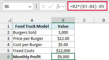
This takes the profit on each burger (price minus cost), multiplies it by the burgers sold, and subtracts the fixed costs. With the current inputs, the truck makes $9,000 a month.

Data Tables and Scenario Manager work in Excel 365, 2024, 2021, 2019, and 2016. In Excel for the web you can view the results, but you need the desktop app to create them.

One-Way Sensitivity Analysis Using a Data Table (Recommended)

Let’s start with the simplest question. What happens to profit if only one input changes and everything else stays as it is?

This is called one-way sensitivity analysis, and I recommend a one-variable Data Table for it because it runs your own model for every value you want to test. Let me show you how it works.

Below is the food truck model with a list of prices, and I want to get the monthly profit at each price in column E.

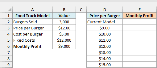
The Data Table needs to know which result to track, so that comes first. Enter this formula in cell E2, which is one row above the first price and one column to its right:

=B6

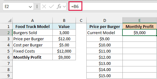
The Current Model label in D2 is only there to tell you what E2 is showing. Excel doesn’t use that cell.

Here are the steps to fill in the rest of the table:

1. Select cells D2:E9.

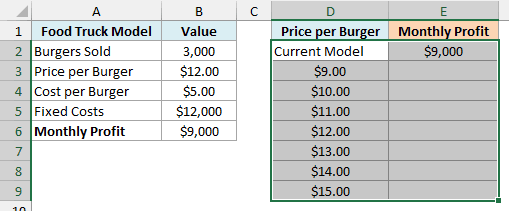
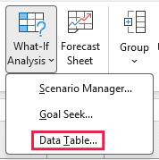
2. Click the Data tab, then click What-If Analysis, then click Data Table.

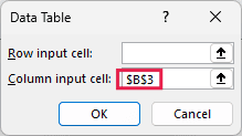
3. Click in the Column input cell field and select cell B3. Leave Row input cell empty.

4. Click OK.

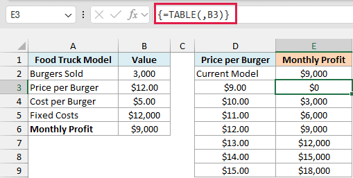
At $9 the truck just breaks even, and every extra dollar on the price adds $3,000 to the monthly profit.

I used the Column input cell because the prices run down a column, and B3 is the price cell in the model.

The input cell has to be on the same sheet as the Data Table, so keep your list next to the model. If it’s on another sheet, Excel stops with “Input cell reference is not valid.”

Also, make sure you pick a cell the model actually uses. If you pick one it doesn’t use, you get no error, just the same profit in every row.

How does this work?

Excel takes each price from column D and puts it into B3 behind the scenes. It then reads the answer from E2 and writes it next to that price, while your real B3 stays at $12 the whole time.

If you click any result, the formula bar shows {=TABLE(,B3)}. The empty spot before the comma is the row input cell, which this table doesn’t use, and B3 is the column input cell.

That formula belongs to the whole table, so if you try to delete just one result, Excel tells you it can’t change part of a data table. To remove the results, select all of E3:E9 and press Delete.

The table normally updates by itself when you change something in the model. Large Data Tables can slow a workbook down though, which is why Excel has a calculation setting that leaves them out.

Important: If your table isn’t updating, go to Formulas > Calculation Options and check if Automatic Except for Data Tables is selected. The table then keeps its old numbers until you press F9 or switch back to Automatic.

Two-Way Sensitivity Table Using a Data Table

Price rarely moves alone. If you raise it, you’ll probably sell fewer burgers, so it helps to see both inputs together.

A two-way sensitivity table does that, with one input down the side and the other across the top. You build it with a two-variable Data Table, and the only setup change is where the formula goes.

Below is the same model with prices down column D and burger counts across row 2, and I want to get the monthly profit for every combination in E3:I9.

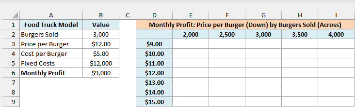
This time the result formula goes in the corner, where the prices and the burger counts meet. Enter this formula in cell D2:

=B6

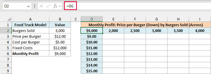
Here are the steps to fill in the table:

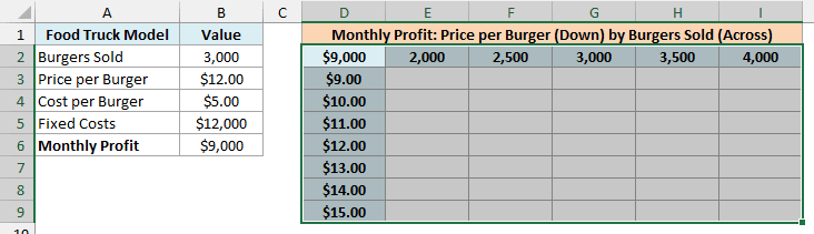
1. Select cells D2:I9.

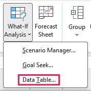
2. Click the Data tab, then click What-If Analysis, then click Data Table.

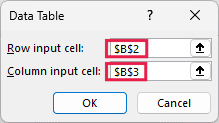
3. Select cell B2 for Row input cell and cell B3 for Column input cell.

4. Click OK.

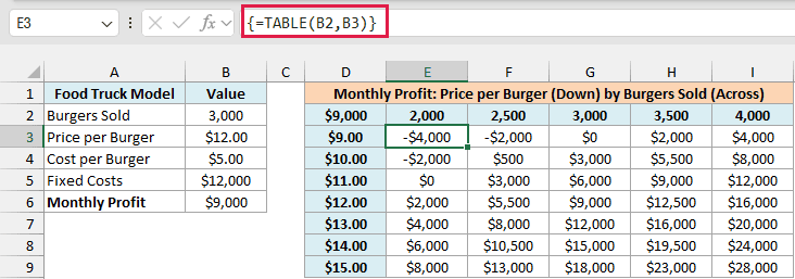
The row input cell is for the values across the top row, which are burger counts here, so it points to B2. The column input cell is for the values down the side, which are prices, so it points to B3.

Important: If you swap the two input cells, Excel gives no error, just wrong numbers. In this table, E3 would show $5,955 instead of -$4,000.

To check your table, find the cell where the current inputs meet, which is G6 here ($12 and 3,000 burgers). It should match the $9,000 in your model.

To spot the combinations that lose money, you can flag them with conditional formatting.

5. Select cells E3:I9, then click the Home tab, then Conditional Formatting, then Highlight Cells Rules, then Less Than.

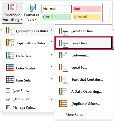
6. Enter 0 in the box and click OK.

The three red cells are the combinations that lose money, and the worst is -$4,000 at $9 with 2,000 burgers. The two $0 cells are exactly break-even, so they stay unflagged.

Two-Way Sensitivity Table With One Formula

If you have Excel 365, 2024, or 2021, you can get the same numbers with a single formula and no Data Table. Below is the same model and layout, and I want to get the monthly profit for every combination in E3:I9.

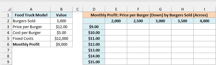
Here is the formula to enter in cell E3:

=E2:I2*(D3:D9-B4)-B5

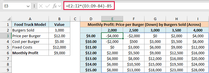
How does this formula work?

D3:D9-B4 gives the profit per burger at each of the seven prices. Multiplying that by the five burger counts in E2:I2 gives one result for every combination, and subtracting B5 takes off the fixed costs.

The result spills across all of E3:I9 from that one cell. The numbers are the same as the Data Table’s.

The catch is that this formula repeats the model’s math, so if the model in B6 changes, you have to update this formula too. A Data Table simply reads B6, which makes it the better choice for a bigger model.

If you’re on Excel 2019 or earlier, use the Data Table above.

Compare Best and Worst Cases Using Scenario Manager

A Data Table stops at two inputs. When you want to change more of them together, like a bad month where you sell less, ingredients cost more, and fixed costs go up, you can use Scenario Manager.

It saves a set of input values under a name, so you can switch the model between them and compare the results in one report.

Below is the food truck model with three sets of input values beside it, and I want to save each set as a scenario and compare the monthly profit on a new sheet.

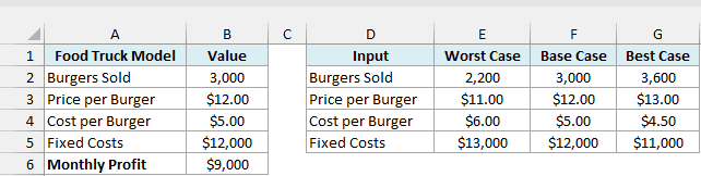
Before adding the scenarios, it’s worth naming the model cells. Without names, the final report labels its rows with cell addresses like $B$3, which are hard to read.

Here are the steps to name the cells and add the scenarios:

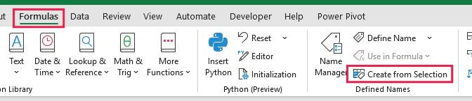
1. Select cells A2:B6, then click the Formulas tab, then click Create from Selection.

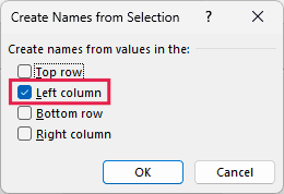
2. Check only Left column and click OK.

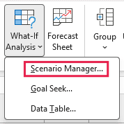
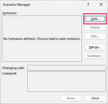
3. Select cells B2:B5, then click the Data tab, then What-If Analysis, then Scenario Manager.

4. Click Add.

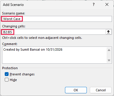
5. Type Worst Case as the scenario name, make sure Changing cells shows B2:B5, and click OK.

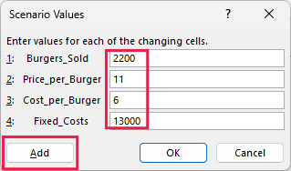
6. Enter the Worst Case values (2200, 11, 6, and 13000) and click Add.

7. Add Base Case and Best Case the same way, using the values from the table. Click OK instead of Add after the last one.

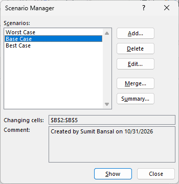
Your three scenarios are now saved in the workbook. To see one in the model, you can select it and show it.

8. Select Worst Case and click Show.

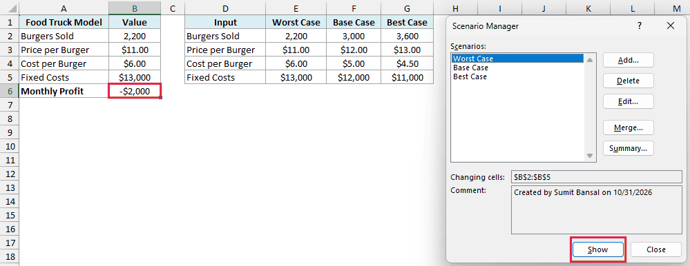
The model now shows a loss of $2,000 in B6, because Excel has written the Worst Case values into B2:B5.

Important: Show replaces the values in your input cells, and the model stays on whichever scenario you showed last. That’s why I saved the original numbers as Base Case, so you can always go back to them.

Here are the steps to go back to the original numbers and create the summary report:

9. Select Base Case, click Show, and then click Summary.

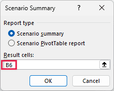
10. Keep Scenario summary selected, enter B6 in Result cells, and click OK.

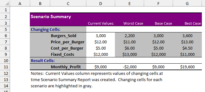
Excel puts the report on a new sheet called Scenario Summary. Monthly profit runs from -$2,000 in the worst case to $19,600 in the best case, with the base case at $9,000.

This report is a snapshot and has no formulas in it. If you change a scenario or the model later, the report keeps its old numbers, so you need to click Summary again to create a new one.

Make a Tornado Chart to See Which Input Matters Most

So far we’ve seen what happens when inputs change. A tornado chart answers a different question, which is which input moves the result the most.

Each input gets one line with two bars running in opposite directions from the current profit. The input with the biggest swing goes on top and the smallest at the bottom, so the chart ends up shaped like a tornado.

Excel doesn’t have a built-in tornado chart, but a clustered bar chart with a few changes gets you there.

Below is the food truck model with its four inputs listed in column D, and I want to find out how much the profit swings in column J when each input moves up or down by the percentage in B8.

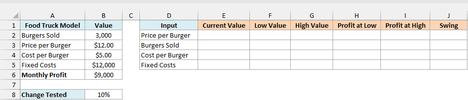
First, link each input to the model in column E. Here is the formula for the price in cell E2:

=$B$3

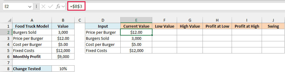
The other three rows follow the same idea, =$B$2 for burgers sold, =$B$4 for the cost per burger, and =$B$5 for fixed costs.

The dollar signs matter because the chart needs this table sorted later, and absolute references keep pointing to the right cells when the rows move.

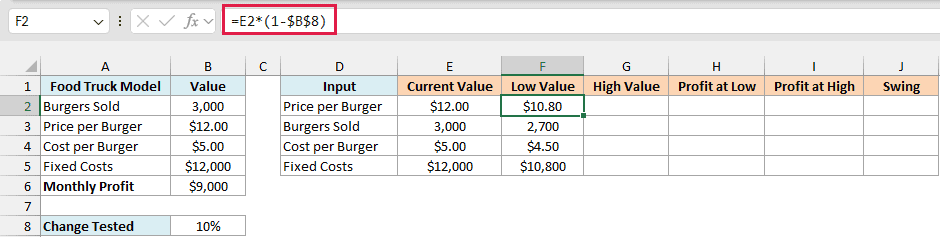
Next, get the low value for each input. Enter this formula in cell F2 and copy it down to F5:

=E2*(1-$B$8)

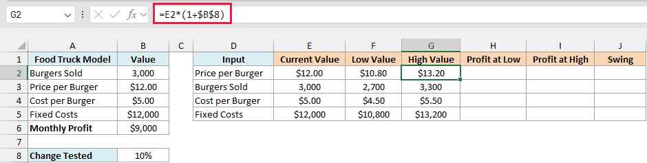
Then get the high value. Enter this formula in cell G2 and copy it down to G5:

=E2*(1+$B$8)

We’re keeping these per-row instead of using a single spilling formula because Excel won’t sort a table that contains a spill.

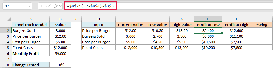
Now calculate the profit at each low value. Each row needs its own formula because each row changes a different input, so it’s the model’s formula with one input swapped for column F.

Enter these in H2:H5:

• Price per Burger, in H2: =$B$2*(F2-$B$4)-$B$5
• Burgers Sold, in H3: =F3*($B$3-$B$4)-$B$5
• Cost per Burger, in H4: =$B$2*($B$3-F4)-$B$5
• Fixed Costs, in H5: =$B$2*($B$3-$B$4)-F5

Then copy H2:H5 across to I2:I5. F changes to G when you copy, so the same formulas now use the high values.

The last column is the swing, which is the gap between the two profits. Enter this formula in cell J2 and copy it down to J5:

=ABS(I2-H2)

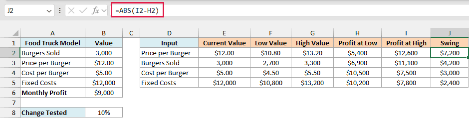
I have used the ABS function because the profit at the high value is lower for the two cost inputs, and a plain subtraction would turn their swing negative.

Price has the biggest swing at $7,200 and fixed costs the smallest at $2,400, so this table is already in the right order. If yours isn’t, select D1:J5, click Data and then Sort, and sort by Swing from largest to smallest.

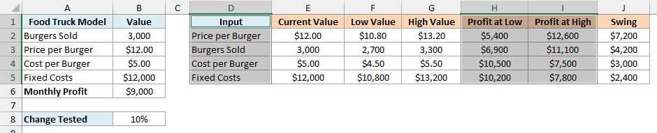
The chart only needs the input names and the two profit columns, which gives each input a Profit at Low bar and a Profit at High bar.

Here are the steps to turn this table into a tornado chart:

1. Select cells D1:D5, hold the Ctrl key, and select cells H1:I5.

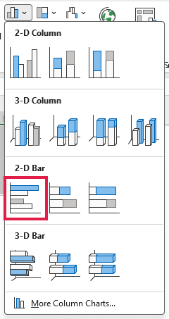
2. Click the Insert tab, then Insert Column or Bar Chart, then Clustered Bar.

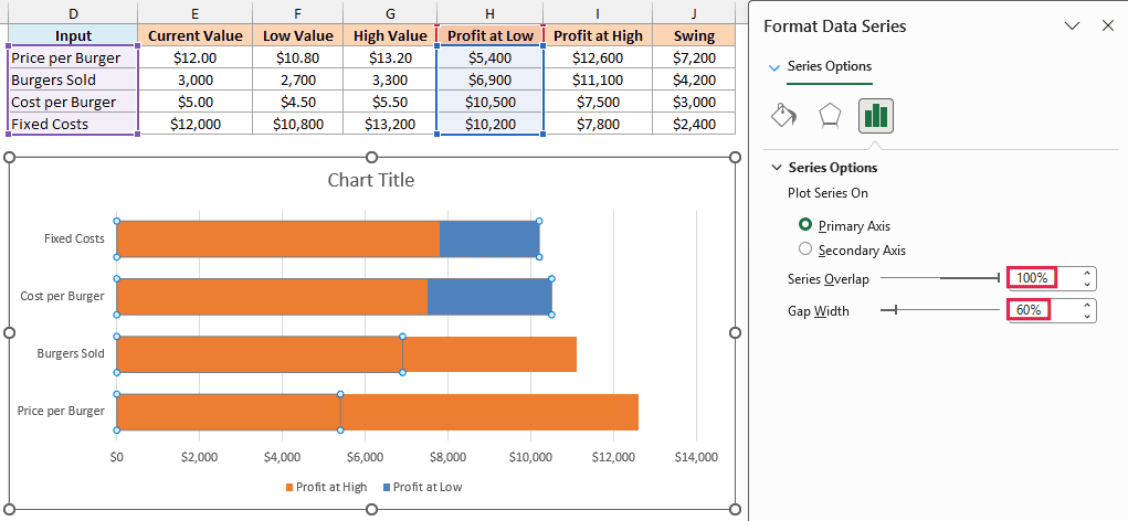
3. Right-click any bar, click Format Data Series, and set Series Overlap to 100% and Gap Width to 60%.

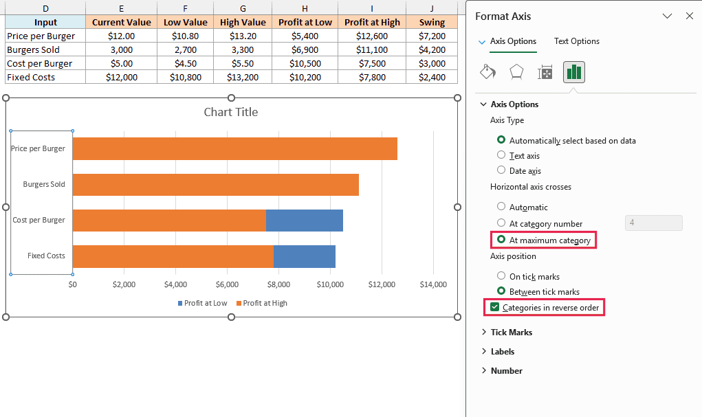
4. Click the vertical axis with the input names. In the pane, check Categories in reverse order and select At maximum category under Horizontal axis crosses.

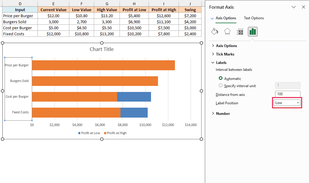
5. In the same pane, expand Labels and set Label Position to Low.

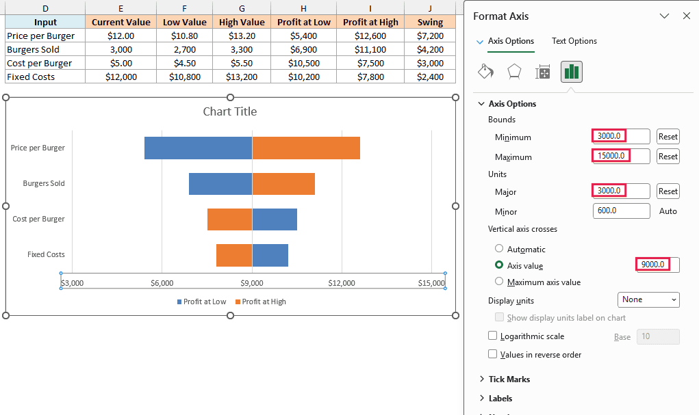
6. Click the horizontal axis with the dollar values. In the pane, set Minimum to 3000, Maximum to 15000, and Major to 3000, then set Vertical axis crosses to Axis value 9000.

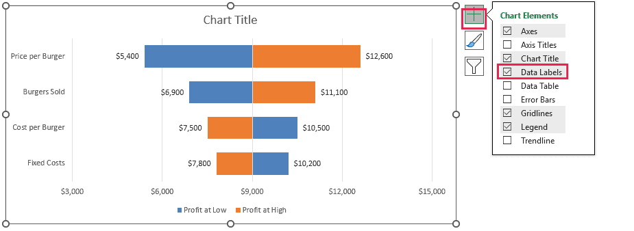
7. Click the Chart Elements button (the plus sign next to the chart) and check Data Labels.

8. Click the chart title and type Monthly Profit When Each Input Moves Up or Down.

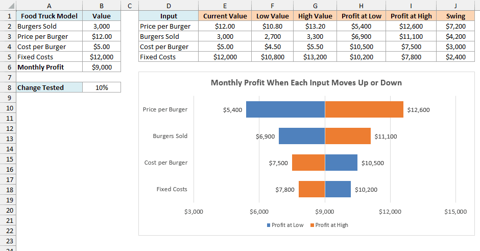
A Series Overlap of 100% puts each input’s two bars on one line instead of side by side. Categories in reverse order puts the biggest swing on top, because a bar chart otherwise starts from the bottom.

Reversing the order also moves the dollar axis to the top of the chart, and At maximum category brings it back down. Setting Label Position to Low keeps the input names on the left instead of on top of the bars.

The 9000 in step 6 is the current profit, and it’s what makes the bars grow left and right from the middle of the chart.

Those axis numbers are typed in though, so if you change the model or the percentage in B8, you’ll need to update them. Set the crossing value to the new profit in B6.

Then pick a Minimum and Maximum that fit the lowest and highest profits in H2:I5, with the current profit in the middle. Major sets the gap between the dollar labels, so pick one that lands a label on the current profit.

A 10% miss on the price moves profit three times as much as a 10% miss on fixed costs, so the price is the estimate worth checking first.

Also notice that the Profit at Low bar is on the right for Cost per Burger and Fixed Costs. That’s correct, because lower costs mean higher profit.

So these are the ways you can do sensitivity analysis in Excel, using one-way and two-way Data Tables, Scenario Manager, and a tornado chart.

I hope you found this article helpful.

Other Excel Articles You May Also Like:

• Data Analysis [Part 4 of 5] – Goal Seek in Excel
• Data Analysis [Part 5 of 5] – Using Solver in Excel
• How to Forecast in Excel (Formulas & Forecast Sheet)