

If you want to calculate the factorial of a number in Excel, you don’t need to take out your pen and paper. A simple formula would do that for you.
I was kind of a math nerd in school, and the sections about probability and permutation/combination were among my favorites. I remember spending a lot of time calculating factorials as a part of the probability calculations.
Excel has the in-built FACT function that can be used to calculate the factorial of any number.
In Excel 365, Excel 2024, and Excel 2021, you can also feed FACT a whole range and the results spill into the cells below.
In this article, I’ll show you how to use the FACT function, with examples covering permutations, combinations, and the errors you may run into.
What is a Factorial?
If you already know this and are here just to know how to calculate it in Excel, jump to the next section.
In mathematics, the factorial of a number is the result you get when you multiply that same number with all the integers after it till 1.
For example, the factorial of 5 would be 120 (54321).
A factorial is written as the number with an exclamation sign after it. So the factorial of 5 would be written as 5! (and the value of this would be 120).
FACT Syntax
Here is the syntax of the FACT function:
=FACT(number)
The FACT function only takes one argument:
- number – The nonnegative number for which you want the factorial. If the number has a decimal part, FACT truncates it to a whole number first.
FACT works in Excel for Microsoft 365, Excel 2024, 2021, 2019, 2016, and older versions, plus Excel on the web.
Let me show you a few practical examples of how to use this function.
Example 1: Calculate the Factorial of a Number
Let’s start with the simplest case.
I want the factorial of 5, which means multiplying 5 by every whole number below it, down to 1.
Here is the formula:
=FACT(5)
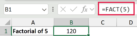
This gives me 120, which is 54321.
Typing the number straight into the formula like this works well when it’s a one-off calculation.
Example 2: Calculate Factorial for a Column of Numbers
Here’s a more practical scenario.
Below is the dataset. Column A has the number of tracks in a playlist, going from 1 up to 8.
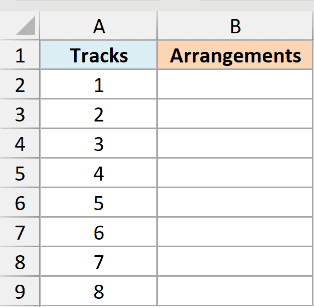
I want to know how many different orders each playlist could be played in.
Here is the formula:
=FACT(A2)
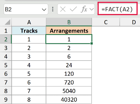
A playlist of 8 tracks can be played in 40,320 different orders. That’s what a factorial counts: the number of ways you can arrange a set of distinct items.
Instead of copying that formula down, you can hand FACT the entire range in one go:
=FACT(A2:A9)
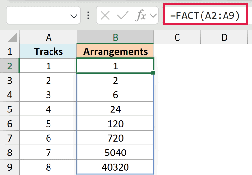
One formula, and the results spill into the cells below on their own. This works in Excel 365, Excel 2024, and Excel 2021.
Pro Tip: If anything is already sitting in the cells where the results need to land, the formula returns a #SPILL! error. Clear those cells and the results appear right away.
Example 3: Calculate Permutations Where the Order Matters
Let me show you an example where calculating factorial might be required, right out of my school math textbook.
Let’s say I have 5 different colored balls with me, and I want to find out how many pairs of different colored balls I can make, where the order of the colors matters. Red and Green would be different from Green and Red.
The mathematical formula for this is 5!/(5-2)!, which works out to 5!/3!.
Here is the formula:
=FACT(5)/FACT(3)
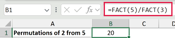
This returns 20.
Here’s why it works. There are 5 balls you could pick first and 4 left to pick second, so 5*4 = 20.
Dividing 5! by 3! is what gets you there. The 3! cancels out all the arrangements of the 3 balls you didn’t pick.
Pro Tip: Excel has a PERMUT function that does this in one step. =PERMUT(5,2) also returns 20, and you don’t have to work out the n!/(n-r)! part yourself.
Example 4: Calculate Combinations Where the Order Doesn’t Matter
Now let’s flip that question around.
Same 5 colored balls, but this time the order doesn’t matter. Red and Green counts as the same pair as Green and Red, so I want to know how many unique pairs I can make.
The mathematical formula for this is 5!/(2!*3!).
Here is the formula:
=FACT(5)/(FACT(2)*FACT(3))

This returns 10.
It’s the permutation answer from Example 3, divided by 2!. Every pair got counted twice there (once as Red-Green and once as Green-Red), and dividing by 2! removes that double counting.
Pro Tip: In case you want to calculate unique combinations in Excel, you can use the COMBIN function instead. =COMBIN(5,2) returns the same 10 without the long division.
Example 5: What FACT Does With Decimals, Zero, and Negatives
This last one is less of a use case and more of a “good to know”.
Below is the dataset. Column A has four values I want to run through the FACT function: 5, 5.6, 0, and -1.
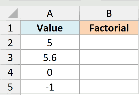
I want to see what FACT returns for each of these.
Here is the formula:
=FACT(A2)
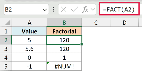
I’m keeping this one per-row so you can see each result sitting right next to the value that produced it.
Here is what comes back:
=FACT(5)returns 120, as expected.=FACT(5.6)also returns 120. The argument needs to be an integer, so if you enter a number that has a decimal part, the formula only considers the integer part.=FACT(0)returns 1. That’s not a quirk of Excel, it’s the mathematical definition of 0!.=FACT(-1)returns the #NUM! error. FACT needs a nonnegative number, so a negative one gives you an error.
Tips & Common Mistakes
- FACT truncates, it doesn’t round.
=FACT(5.9)gives you 120, which is the factorial of 5. It does not round up to 6 and give you 720. - If a cell reference could hold a negative value, wrap the formula in IFERROR so the reader sees a message instead of the #NUM! error code.
- There is an upper limit.
=FACT(170)returns roughly 7.26E+306, which is about as large a number as Excel can hold.=FACT(171)gives the #NUM! error because the result is bigger than that. - Once a factorial runs past 15 significant digits, Excel stores a rounded version of it. So treat the tail end of a huge factorial as a ballpark, not an exact count.
So this is how you can easily calculate factorial in Excel.
I hope you found this formula tutorial useful!
Other Excel Articles You May Also Like:
