Create All Possible Combinations from Lists in Excel

I was recently working on a project where I had multiple lists in Excel and I had to create all the possible combinations using these lists.

To give you an example, suppose I three separate lists where I have:

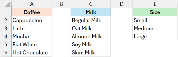
• 5 type of coffee
• 5 types of Milk
• 3 different cup sizes

Now I want to get one single list that would include all the possible combinations from these three lists above. This would give me a total of 75 combinations (5 x 5 x 3) as shown below.

There are multiple ways you can tackle this situation in Excel. The easiest ways to use Power Query that will do this with a few clicks, and in case the data changes then you can easily refresh the query and get the updated result.

I’ll also show you how to do this using an Excel formula as well as VBA.

Generate All Combinations Using Power Query

Below I have a dataset where I have three lists – 5 types of coffee, 5 types of milk, and 3 different cup sizes.

I want to generate all possible combinations from these three lists.

Let’s see how to do this using Power Query.

Step 1 – Convert all lists to Excel Tables

To use our lists in Power Query, we first need to convert all of them into Excel Tables.

Below are the steps to do this:

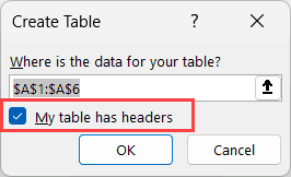
1. Select any cell within your coffee list and press Ctrl+T. Alternatively, you can also click on the Insert tab in the ribbon and then click on Table

2. In the Create Table dialog box that opens, make sure the “My table has headers” option is checked, then click OK.

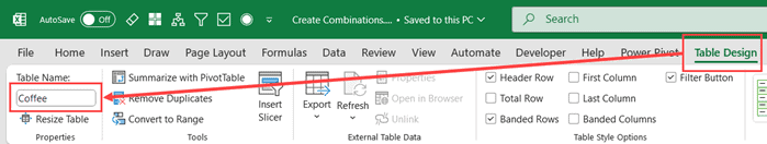
3. Rename this table by click on the Table Design tab and then changing Table Name. In this case, I will rename it to Coffee

Repeat the same process for the Milk list (rename the table to “Milk”) and the Sizes list (rename the table to “Sizes”).

Step 2 – Open Each List in Power Query and Save as Connection

Now that we have these tables in Excel, we will open them one by one in Power Query and save them as connections.

We are doing that to make these lists avaialble in Power Query so that we can them combine them.

Here is how to do this:

1. Select any cell in the Coffee Table
2. Go to the Data tab and click on “From Table/Range” icon (it’s in the Get & Transform section). This will open the Power Query editor with your Coffee table.

3. Click on the File tab, and then click on the Close and Load To option

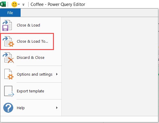
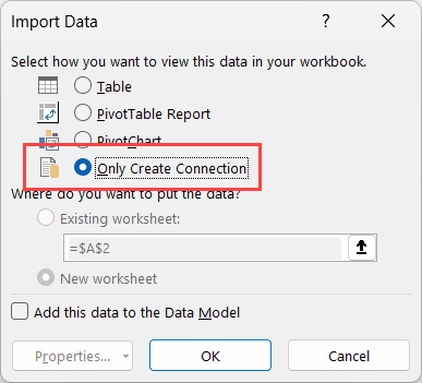
4. In the Import Data dialog box, select the Only Create Connection option and then click OK

Repeat this same process for the milk and sizes tables. You should now see all three connections in the Queries & Connections pane.

Step 3 – Create New Query to Combine all the Lists

Now that we have all the three lists in power query as connections we are going to create a new query that would combine all the three lists and give us all the possible combinations.

This new query that we create is the one that we will load into our worksheet to get the result.

Here are the steps to do this:

1. Press Alt+F12 to open a blank Query in the Power Query editor.
2. In the Query Navigation pane, right-click and select New Query > Other Sources > Blank Query.

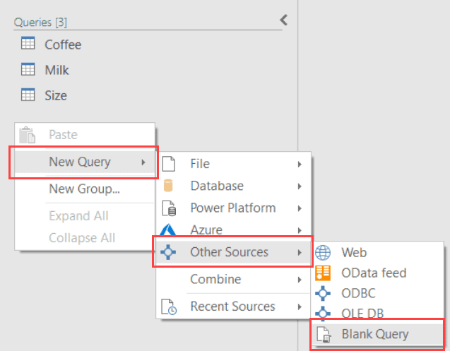
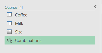
3. Rename this query as “Combinations”.

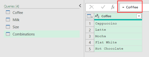
4. In the formula bar, type “Coffee” and and click in the area below it. This will bring in your coffee data within this new query.

5. Now click Add Column option in the ribbon and then click on Custom Column. This will open the Custom Column dialog box.

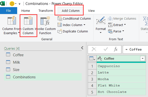
6. In the Custom column formula field, enter the following:

=Milk

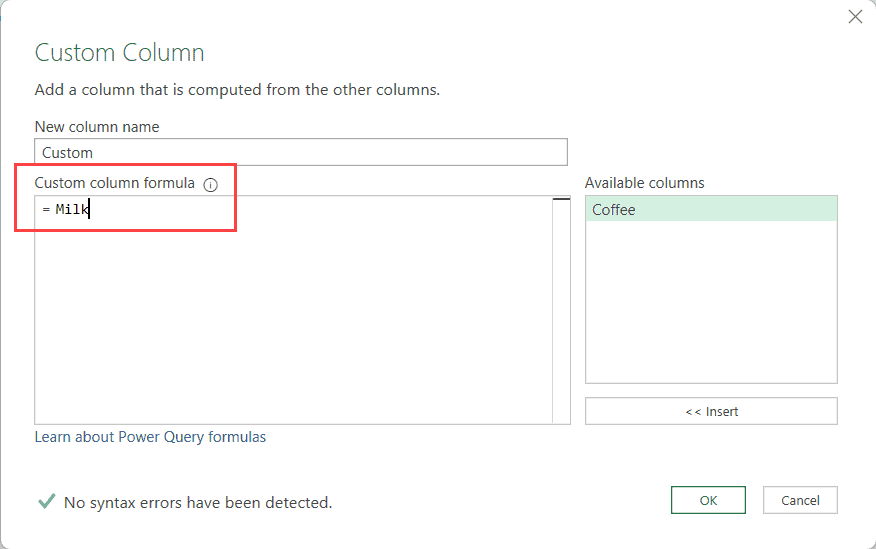
7. Click OK

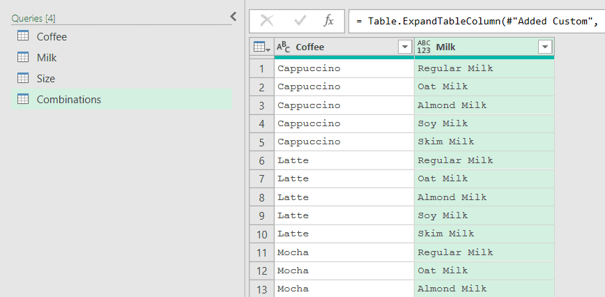
This is the step where magic happens. Doing this would add the milk table in each row in the already existing coffee table. You will see a new column that appears has Table as the value in each cell. This means that every cell holds the Milk table in each cell

8. Click the expand button (double arrows) in the column header of the newly added column and uncheck “Use original column names as prefix” option and then click OK.

After this step you would have a two column table that gives you all the possible combinations of coffee and milk type lists

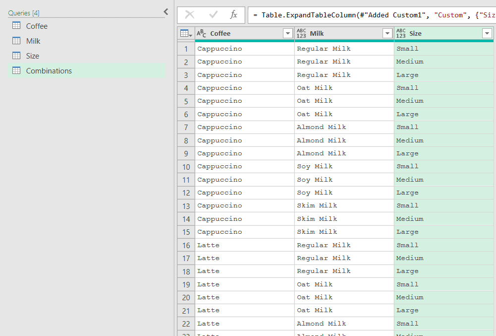
9. Repeat steps 5-7 for the Sizes list. Add a custom column with “Sizes” as the formula, then expand it.

Once you’re done with the above steps, you’ll now have 75 records (5 coffee types × 5 milk types × 3 sizes) with all possible combinations.

But we still have this data in our query and we need to load it back into Excel

Step 4 – Load The Combinations Query into Excel Worksheet

Here are the steps to load this table in Power Query editor into Excel:

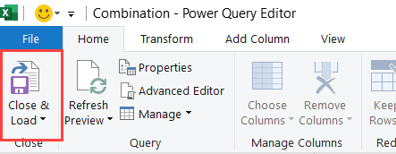
1. Go to Home tab in the Power Query Editor
2. Click on the “Close & Load” option.

This will add a new worksheet in the workbook and give you the resulting data as an Excel Table.

If you make changes to any of your original lists (like adding a new size), you can simply refresh the query (right-click on the query and select Refresh), and your combinations table will update automatically.

Generate All Combinations Using Formula

While Power Query is a better and more robust way to generate all combinations from two or more lists, if you want to do this using formulas let me give you one.

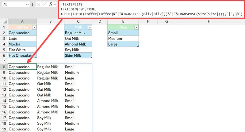
Below I have three Excel tables that contain different types of Coffee, Milk types, and Sizes and I want to generate all possible combinations from these three lists.

I have named these tables as Coffee, Milk, and Size respectively.

Here is the formula that will give you all the possible combinations from all the lists:

=TEXTSPLIT(TEXTJOIN("@",TRUE,TOCOL(TOCOL(Coffee[Coffee]&"|"&TRANSPOSE(Milk[Milk]))&"|"&TRANSPOSE(Size[Size]))),"|","@")

The above formula uses a combination of TOCOL and TRANSPOSE to give us unique combinations from all the lists.

For example, the below part of the formula would give us a list that would list a unique combination in a cell separated by a pipe symbol.

=TOCOL(TOCOL(Coffee[Coffee]&"|"&TRANSPOSE(Milk[Milk]))&"|"&TRANSPOSE(Size[Size]))

Now to split it into separate cells, I have used the TEXTJOIN function that first combines the entire list into one single string and then splits it based on the delimiter into columns and rows.

If you want to learn why I’ve done this and how this formula works, you can watch the below video:

In the above video, I’ve taken the same example and I’ve shown two ways to use a formula to get the result.

Also read: Repeat Rows N Times in Excel

Generate All Combinations Using VBA

If, for some reason, you do not want to use power query and do not have access to these new Excel functions, you can use vba to quickly generate all possible combinations.

Below the VBA code that I have created that generates all possible combinations and then insert it as an Excel table in a newly inserted worksheet (called Combinations).

You can modify the code according to your need (such as adjusting the references and column names)

'Code by Sumit Bansal from TrumpExcel.com

Sub GenerateCombinations()
    ' Declare variables
    Dim coffeesRange As Range, milksRange As Range, sizesRange As Range
    Dim coffee As Range, milk As Range, size As Range
    Dim outputSheet As Worksheet
    Dim currentRow As Long
    Dim totalCombinations As Long
    
    ' Define input ranges (adjust these ranges to match your actual data)
    Set coffeesRange = Sheets("Sheet1").Range("A2:A6")  ' Coffee types in column A
    Set milksRange = Sheets("Sheet1").Range("C2:C6")    ' Milk types in column C
    Set sizesRange = Sheets("Sheet1").Range("E2:E4")    ' Sizes in column E
    
    ' Create or activate output sheet
    On Error Resume Next
    Set outputSheet = Sheets("Combinations")
    If outputSheet Is Nothing Then
        Set outputSheet = Sheets.Add(After:=Sheets(Sheets.Count))
        outputSheet.Name = "Combinations"
    End If
    On Error GoTo 0
    
    ' Clear any existing data
    outputSheet.Cells.Clear
    
    ' Create headers
    outputSheet.Range("A1").Value = "Coffee"
    outputSheet.Range("B1").Value = "Milk"
    outputSheet.Range("C1").Value = "Size"
    outputSheet.Range("A1:C1").Font.Bold = True
    
    ' Calculate total combinations for progress reporting
    totalCombinations = coffeesRange.Cells.Count * milksRange.Cells.Count * sizesRange.Cells.Count
    
    ' Start with row 2 (row 1 has headers)
    currentRow = 2
    
    ' Generate all combinations
    Application.ScreenUpdating = False
    
    ' Display progress bar
    Application.StatusBar = "Generating combinations... Please wait."
    
    ' Loop through all combinations
    For Each coffee In coffeesRange.Cells
        For Each milk In milksRange.Cells
            For Each size In sizesRange.Cells
                ' Add combination to output sheet
                outputSheet.Cells(currentRow, 1).Value = coffee.Value
                outputSheet.Cells(currentRow, 2).Value = milk.Value
                outputSheet.Cells(currentRow, 3).Value = size.Value
                
                ' Move to next row
                currentRow = currentRow + 1
                
                ' Update status bar with progress
                If currentRow Mod 10 = 0 Then
                    Application.StatusBar = "Generating combinations... " & _
                        Format((currentRow - 2) / totalCombinations, "0%") & " complete"
                    DoEvents
                End If
            Next size
        Next milk
    Next coffee
    
    ' Format as table for easy filtering
    outputSheet.Range("A1:C" & currentRow - 1).Select
    outputSheet.ListObjects.Add(xlSrcRange, outputSheet.Range("A1:C" & currentRow - 1), , xlYes).Name = "CoffeeCombinations"
    
    ' Auto-fit columns
    outputSheet.Columns("A:C").AutoFit
    
    ' Reset status bar and screen updating
    Application.StatusBar = False
    Application.ScreenUpdating = True
    
    ' Inform user of completion
    MsgBox "Generated " & (currentRow - 2) & " combinations.", vbInformation
    
    ' Select cell A1 in the output sheet
    outputSheet.Range("A1").Select
End Sub

To use this code, open the VB editor, insert a new module, and copy paste the above code into it. Once done, make any adjustment in the code (as needed) and then run it.

Note: Since the change is done by VBA codes are irreversible, always ensure that you have a backup copy of your file (in case anything goes wrong)

In this article I showed you three different ways you can use to generate all possible combinations from two or more lists.

Power Query as the best and most robust solution among the three. While there are a few steps in the initial setup once you have it ready it’s super easy to refresh your result in case any of the list changes.

I’ve also covered a formula method and a VBA code method in case there’s a situation where you cannot use Power Query.

I hope you found this article helpful.

In case you have any questions or you know of any other method that can be used to generate all possible combinations, do let me know in the comments section.

Other Excel articles you may also like:

• CONCATENATE Excel Range (with and without separator)
• Random Group Generator Template [FREE Download]
• How to Combine Cells in Excel
• Generate Random Numbers