If you’re a teacher or a trainer, creating groups of students/participants is a common task. For example, you may want to create groups to conduct a quiz or a team building activity.
And in most of the cases, you need these groups to be random.
Today, I am sharing a random group generator template that will make it super easy for you to create a group of students/participants.
All you need is the list of students or participants and specify how many groups you want to create.

Random Group Generator Template
Here is a demo of how this random group generator (or random team generator) template works:
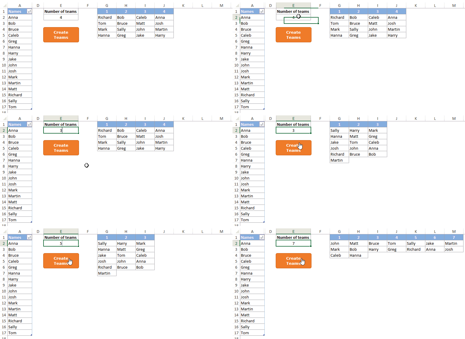
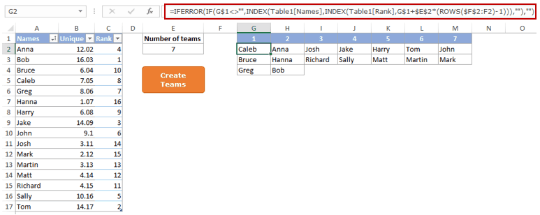
The list of students/participants is in A2:A17. If you have a longer list, simply add the names in it.
Cell E2 has the number of groups that you want to create. Based on the number you enter, you would get the groups and the names in each group in columns G to P. As of now, I have created it this template for a maximum of 10 groups.
Once you have entered the number of groups you want in cell E2, click on the ‘Create Teams’ button to randomly generate the groups of names.
Download the Random Group Generator Template
How this Excel Template Works
There are a couple of cool Excel features and a few helper columns that make this random group generator template in Excel.
Here is how it is made:
- A2:A17 contains the list of names that are to be grouped randomly.
- A1:C17 has been converted into an Excel Table. This helps to keep the formulas intact when you add/remove names from the list.
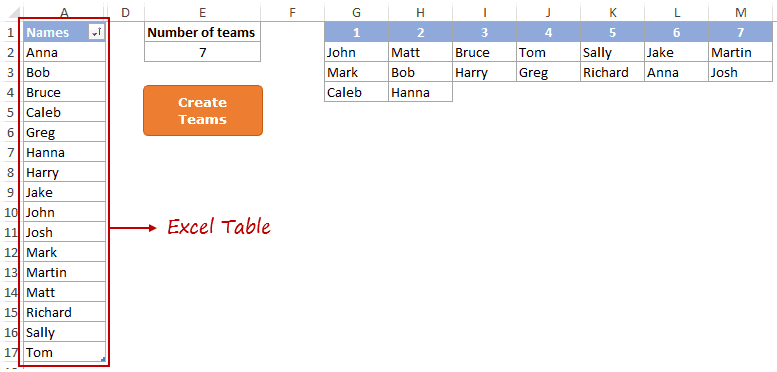
- Column B has the formula: =RANDBETWEEN(1,COUNTA([Names])) + ROW()/100
- The function returns a random number between 1 and the total number of names in the list (using the COUNTA function). To this, ROW()/100 is added to make it unique (as the RANDBETWEEN function can spit out duplicates as well).
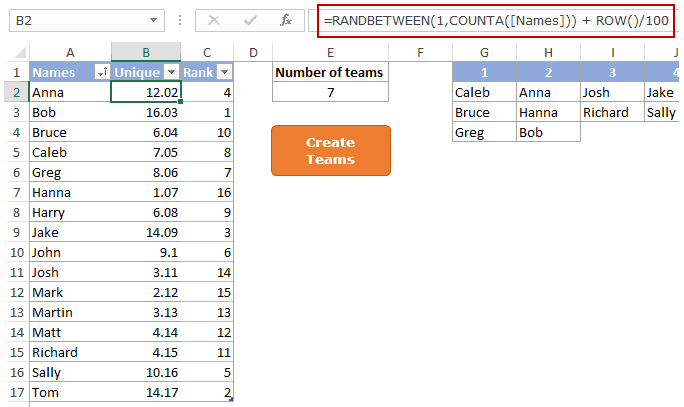
- Cell C2 has the formula: =RANK([@Unique],[Unique])
- This function gives the rank for each value in Column B. Since all the values in column B are unique, this formula gives a unique list of integers that vary from 1 to the total number of names in the list.

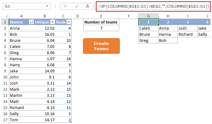
- Cell G1 has the formula: =IF(COLUMNS($G$1:G1)>$E$2,””,COLUMNS($G$1:G1))
- The same formula is copied in cells H1 to P1. It returns the number of columns between column G and the current column. Hence, G1 gets 1, H1 gets 2 and so on. It also checks whether the number is greater than the value in cell E2. If yes, then it returns a blank.
- Cell G2 has the formula: =IFERROR(IF(G$1<>””,INDEX(Table1[Names],INDEX(Table1[Rank],G$1+$E$2*(ROWS($F$2:F2)-1))),””),””)
- It is copied to all the cells in G2:P17.
- In cell G2, this formula will pick up the rank from C2 and return the name at that position in the list.
- In cell G3, it will pick the rank from C6 (which is 1 + 1*4, where 4 is the number of groups to be formed).
- In cell G4, it will pick the rank from C10 (which is 1 + 2*4, where 4 is the number of groups to be formed).
- If the cell in the first row is empty or the result of the formula is an error, it returns a blank.
- It is copied to all the cells in G2:P17.
Since RANDBETWEEN function is volatile, it will automatically refresh every time you make a change in the worksheet. This may be undesirable as it will change the grouping every time.
To avoid this:
- Go to File Options.
- In the Excel Options dialog box, select formulas in the pane on the left.
- In the Calculation options, make Workbook Calculation Manual.
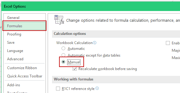
- Click OK.
Now the worksheet would not refresh until you force a refresh by hitting the F9 key.
But to make it look better, there is an orange button that does the refresh when you click it. There is a one-line VBA code at play here that gets executed whenever you click the button.
Here is how to insert this button:
- Go to Developer –> Code –> Visual Basic. (You can also use the keyboard shortcut Alt + F11).

- In the VB Editor right-click on any of the objects for the workbook and go to Insert –> Module.
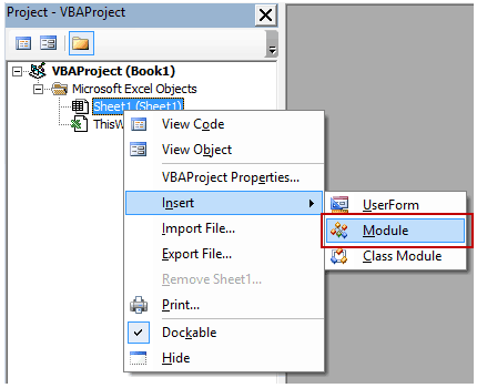
- In the module code window, copy-paste the following code:
Sub Refresh() Worksheets("Team Generator").Calculate End Sub- Note that the name of the worksheet is in double-quotes. If your worksheet name is different, change it in the code.

- Close the VB Editor.
- Go to Insert –> Shapes and insert any shape that you want as the button.
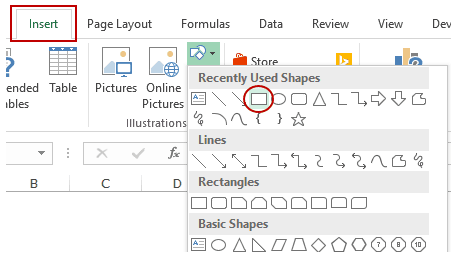
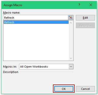
- Right-click on the shape and click on Assign Macro.

- In the Assign Macro dialog box, select the macro name and click on OK.
- Format the button the way you want.
Now when you click on the button, the worksheet would recalculate and you would get a new grouping based on the number of groups you have specified.
Download the Random Group Generator Template
Other Excel Templates You May Like:
- Employee Leave/Vacation Tracker Template.
- Employee Timesheet Calculator.
- Excel To Do Lists Templates.
- A collection of FREE Excel Templates.
- Random Group / Team Generator (Free Tool)
You may also like the following Excel tutorials:


I need to add columns like, Last name, email address, Gender, City, and two more columns. Can you please guide me on how to work on the VBA so that I can use your template?
Is there any way to increase the max number of groups? I really need 15 groups! Please help… would be so great to use in my classroom.
I am sorry but the random team generator isn’t working correctly. It will pull duplicates about every 8th run. Conditional format for dups and you will see. Can it be fixed? I have trying but to no avail. Please advise. M
Thank you …i almost got here myself but couldn’t figure put how to add the names to the teams…awesome!
Thanks for the template! Is there a way to specify that I would want to have my samples distributed randomly across three groups (A,B,C) but have e.g. 80% of them in group-A, 10% in group-B and 10% in group-C?
Doesnt work, can anyone help. Why does the formual reference cell F if there is nothing in it?
You can help me to create a specific random match, is for a sport team, 6 teams with 3 members i need matching with rival teams and similar weight for the member or very close weight , please i pay you
This is a great tool. However I tried modifying it. But could’nt.
I just need 1 Team where I need to mention the no of members in cell E2 and it creates a team with Random Names. I am confident its a piece of cake for you.
Absolutely perfect but I need the absent function to work. I would love to this to randomly select 3 or 4 ball groups of golfers whilst we are on the tee. However we are never sure who is going to turn up hence the need to mark golfers absent from the master list and randomise the selection of the players who are there. Can anyone help???
Sorry this does not work very well.
I have 40 teams and they have to be paired this goes no where needed for this program to work.
Hey there,
Loved this!
i ended up making a few alterations of my own, namely, put the generating function into VBA so that it stopped updating all the time, I added some arrows to increase/decrease the number of groups with a single click and also made a ‘secret’ tab where you could specify two people you didn’t want in the same group. I’d be happy to share it if you’re interested.
Hi Steve,
Please do share how you worked on “secret” tab.
Is there a way to set group 1 to have 10 members, and the others to have like 7 ?
Cool trick, but i have one scenario. let’s say i have names(2 or more) that cannot be teamed together,is there any way to solve it?
Hi Sumit!
This is amazing for my classroom thanks so much!
Is there any way to increase the max number of groups? I really need 12 groups!
Dear Sumit,
I really enjoy using your random group generator for my classes (I created a tab for each class. It’s swift and easy to use.
Sometimes, however someone in a class is absent (visit to the dentist, etc.).
If so, I have to alter the table, to remove the absent student.
It would be nice if there could be a column next to the student names where I could mark the absent student(s) (for example with a zero) , so he/she won’t be displayed in the generated groups.
Unfortunately I don’t have the programming skills to make that happen.
Someone else perhaps?
Greetings,
Willem
(Netherlands)
Thanks Willem.. Glad you liked it.
Here is a link to a new template that will allow you to mark a student as absent: https://www.dropbox.com/s/ys1mmwmbdy7eeb5/Random-Team-Generator-Template%20Absent.xlsm?dl=0
Hi Sumit!
This is amazing for my classroom thanks so much!
Is there any way to increase the max number of groups? I really need 12 groups!
Hello… there is something wrong with the absent function in the worksheet…Even if I indicate that the student is absent, his name will still show in the generated teams list… Also, is there anyway to group 40 people into 2 groups… it seems that the template doesn’t support such a function… thanks and keep up the good work! 🙂
Hello, I was searching for an excel template to create random 4 man teams when I happened upon your template. I downloaded it and tested what I am trying to accomplish, but was having trouble when I found the above link. It gets me a step closer to what I am wanting to do, however, I am trying to accomplish the opposite. I have a list of 71, but I only want to include those I identify as opposed to excluding those that are identified. And I want the teams to be in multiples of 4, but I think if I identify the total number of teams, the template will provide me with teams of 3 or 4. So, I am wondering if a template is available that would provide the capability to include vs exclude? Thanks in advance for your help. Andy.
Thanks to both of you, Sumit and Rudra!
Sumit, I enjoy your formulabased random generator. I have my ovn VBA-generator that I will continue using,but I learned a lot from your reallønn Nice formulas.
Rudra! I’ve never notised the easy way of changing calculation mode. I still miss a warning light when ExCeL is in manual mode. Forgetting to return to aut. Mode has caised me lot f extra work.
From the Custom Quick Access Toolbaar, add “Manual” to the Quick Access Toolbaar and it will show when in Manual mode.
Thanks Hennie, I’ve already adferd it to QAT.
Cool trick Sumit. Thanks for sharing. However there is a short cut to change calculation from ribbon itself. Just go to formula ribbon and click on Calculation Option.
Thanks for sharing Rudra.. That’s definitely the faster way to do this.