If you have a list of numbers, it easy to rank it using the RANK function. However, if you have these numbers within various groups, it could be a challenge to find the rank within the groups.
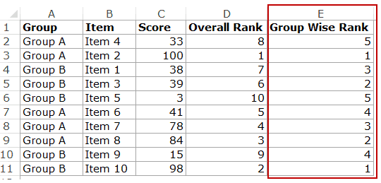
For example, as shown below, there are two groups (A and B) with 5 items in each group. Each item has a score in column C. Now there are two rankings done with this data set. Column D has the overall rankings and Column E has the group-wise rankings.
Now there are two rankings done with this data set. Column D has the overall rankings and Column E has the group-wise rankings.

While the overall ranking can easily be done using the RANK function, the one for groups is a bit more complex.
Rank within Groups in Excel
Here is the formula that will give the ranks within groups in Excel:
=SUMPRODUCT((A2=$A$2:$A$11)*(C2<$C$2:$C$11))+1
How does this work?
This formula checks for 2 conditions:
- (A2=$A$2:$A$11) – This part returns an array of TRUEs/FALSEs based on the group. So if you use this in cell E2, it will check A2:A11 and return TRUE wherever it finds Group A and FALSE when it finds any other group.
- (C2<$C$2:$C$11) – This checks whether the score is less than the other scores in C2:C11, and returns TRUE if it’s less and FALSE if it’s more.
When these two arrays of TRUEs/FALSEs are multiplied, it will return TRUE only in those cases where both the conditions are met, i.e., the group matches and the scores are less than the score in the row where the formula is used.
The SUMPRODUCT formula then simply returns the total count of such instances where the conditions are met.
1 is added to the SUMPRODUCT result to get the rank of the given score within that group.
Click here to download the example file.
I hope you found this tutorial useful!
You May Also Like the Following Excel Tutorials:
- Automatically Sort Data in Alphabetical Order using Formula.
- How to Generate Unique Random Numbers in Excel.
- How to Calculate Age in Excel using Formulas.
- How to Extract a Substring in Excel Using Formulas.
- How to Calculate PERCENTILE in Excel (Easy Formula + Examples)
- Find the Second Largest Value in Excel


If I only want to rank Group A and not Group B. How would that be achieved by either include certain values or excluding certain values?
https://wmfexcel.com/2016/03/12/rank-in-subgroup-rankif/
A similar post using COUNTIFS to solve the problem.
Hope you like it.
We can also use COUNTIFS for ranking in Groups. Formula is
=COUNTIFS($C$2:$C$11,”>=”&C2,$A$2:$A$11,A2)
entering the formula as array formula
{=SUM((A2=$A$2:$A$11)*(C2<=$C$2:$C$11))} gives the same result (typed without the {}'s and entered in the cell with CTRL-SHIFT-ENTER).
Both are able to be expanded as long as data is inserted in the middle or change $11 to $12, in the example formula and insert rows at the last cell of the array before entering new data. The benefit of the C-S-E Array is it has some protection from editing built in.
By the way, above you say the formula ends with "+1", but in the example file, it is not there.
There is another difference in the formula that makes the formula above superior to the formula in the downloaded example – the “<" above is replaced with "<=" in the example – as noted in +1's comment.
For example, a data set with ties using the formula above would result in "1,1,3,4,4,6".
The same data set with the formula in the download would result in "2,2,3,5,5,6".
Hey Jim.. Thanks for pointing out.. I first used the formula with =< without +1, but later found the issue so changed in the tutorial. Forgot to change in the download file. It's fixed now 🙂
You can change the “<" to "=<" (equal or less) in the second multiplier and can then get rid of the "+1."
This will get you the same effect when the items to be ranked are mutually unequal.
When breaking ties is needed, the second formula will get you the upper bound for the rank, which is somewhat unsatisfactory. Perhaps this is what the design with "+1" was chosen in the first place. Too late to delete this comment, though.
Thanks for commenting.. when I first tried, I used “=<" without the +1, but then I compared with the RANK function. So to make it consistent, made it < with +1