How to Generate Random Numbers in Excel

There may be cases when you need to generate random numbers in Excel.

For example, to select random winners from a list or to get a random list of numbers for data analysis or to create random groups of students in class.

In this tutorial, you will learn how to generate random numbers in Excel (with and without repetitions).

Generate Random Numbers in Excel

There are two worksheet functions that are meant to generate random numbers in Excel: RAND and RANDBETWEEN.

• RANDBETWEEN function would give you the random numbers, but there is a high possibility of repeats in the result.
• RAND function is more likely to give you a result without repetitions. However, it only gives random numbers between 0 and 1. It can be used with RANK to generate unique random numbers in Excel (as shown later in this tutorial).

Generate Random Numbers using RANDBETWEEN function in Excel

Excel RANDBETWEEN function generates a set of integer random numbers between the two specified numbers.

RANDBETWEEN function takes two arguments – the Bottom value and the top value. It will give you an integer number between the two specified numbers only.

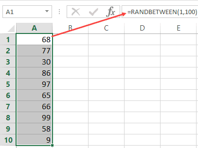
For example, suppose I want to generate 10 random numbers between 1 and 100.

Here are the steps to generate random numbers using RANDBETWEEN:

• Select the cell in which you want to get the random numbers.
• In the active cell, enter =RANDBETWEEN(1,100).
• Hold the Control key and Press Enter.

This will instantly give me 10 random numbers in the selected cells.

While RANDBETWEEN makes it easy to get integers between the specified numbers, there is a high chance of repetition in the result.

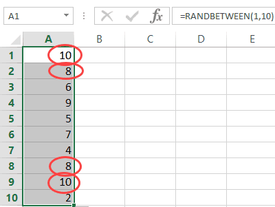
For example, when I use the RANDBETWEEN function to get 10 random numbers and use the formula =RANDBETWEEN(1,10), it gives me a couple of duplicates.

If you’re OK with duplicates, RANDBETWEEN is the easiest way to generate random numbers in Excel.

Note that RANDBETWEEN is a volatile function and recalculates every time there is a change in the worksheet. To avoid getting the random numbers recalculate, again and again, convert the result of the formula to values.

Generate Unique Random Numbers using RAND and RANK function in Excel

I tested the RAND function multiple times and didn’t find duplicate values. But as a caution, I recommend you check for duplicate values when you use this function.

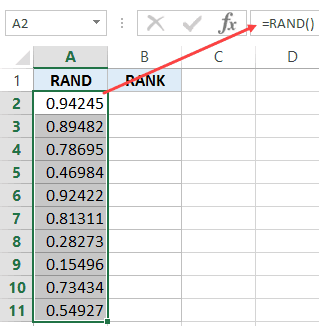
Suppose I want to generate 10 random numbers in Excel (without repeats).

Here are the steps to generate random numbers in Excel without repetition:

• Select the cells in which you want to get the random numbers.
• In the active cell, enter =RAND()
• Hold the Control key and Press Enter.
• Select all the cell (where you have the result of the RAND function) and convert it to values.
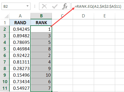
• In the adjacent column, use the following formula: =RANK.EQ(A2,$A$2:$A$11)

Now you can use the values in column B as the random numbers.

Note: RAND is a volatile formula and would recalculate every time there is any change in the worksheet. Make sure you have converted all the RAND function results to values.

Caution: While I checked and didn’t find repetitions in the result of the RAND function, I still recommend you check once you have generated these numbers. You can use Conditional Formatting to highlight duplicates or use the Remove Duplicate option to get rid of it.

You May Also Like the Following Excel Tutorials:

• Automatically Sort Data in Alphabetical Order using Formula.
• Random Group Generator Template
• How to Shuffle a List of Items/Names in Excel?
• How to Do Factorial (!) in Excel (FACT function)