

If you want to find where a piece of text sits inside a longer text string, the SEARCH function is what you’re looking for. It returns the position of the text you’re after, and it does not care about uppercase or lowercase.
In Excel 365, you can also give SEARCH a whole range and the results spill into the cells below. In this article, I’ll show you how to use SEARCH with plenty of practical examples.
Follow along with the example file
SEARCH Function Examples.xlsx
SEARCH Syntax
Here is the syntax of the SEARCH function:
=SEARCH(find_text, within_text, [start_num])
- find_text – the text you want to find the position of.
- within_text – the text in which you want to search for find_text.
- start_num – (optional) the character number in within_text where you want to start searching. If you leave it out, SEARCH starts from the first character. It must be at least 1 and no greater than the length of within_text.
SEARCH returns a number, which is the position of the first character of find_text inside within_text.
When to Use the SEARCH Function
Use SEARCH when you need to:
- Find the position of a character or word inside a text string.
- Locate text without worrying about whether it is upper or lower case.
- Match text patterns using wildcards like
?and*. - Feed a position into functions like LEFT, MID, or RIGHT to pull out part of a string.
- Check whether a cell contains specific text (by pairing it with ISNUMBER).
Let me show you a few practical examples of how this works.
Example 1: Find the Position of a Character
Let’s start with a simple example.
Below is a dataset with product codes in column A. Each code has a dash separating its parts, but the dash sits at a different spot in each code.
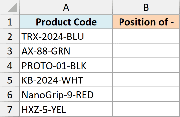
I want to know the position of the first dash in every code.
Here is the formula:
=SEARCH("-", A2:A7)
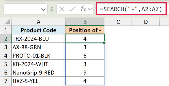
In Excel 365, I only type this once in cell B2. Because I gave SEARCH the whole range A2:A7, the result spills down and returns the dash position for each code.
So for TRX-2024-BLU it returns 4, and for PROTO-01-BLK it returns 6, since that is where the first dash appears in each string.
Example 2: SEARCH Is Not Case-Sensitive (SEARCH vs FIND)
Here is where SEARCH really shines.
Below is a dataset of report titles in column A. Notice that the word “sales” shows up in a different case in each title (Sales, sales, SALES).
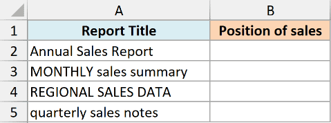
I want to find the position of “sales” in each title, no matter how it is capitalized.
Here is the formula:
=SEARCH("sales", A2:A5)
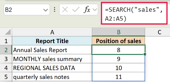
SEARCH finds the word in every title and returns its position. It ignores the case completely, so “sales” matches Sales, SALES, and sales all the same.
Now compare that with the FIND function, which does the same job but is case-sensitive.
Here is the same lookup with FIND, spilled down all four titles:
=FIND("sales", A2:A5)
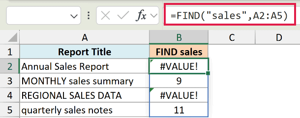
FIND only matches lowercase “sales” exactly. It returns the position in “MONTHLY sales summary” (9) and “quarterly sales notes” (11), where “sales” is written in lowercase. For “Annual Sales Report” (which has “Sales”) and “REGIONAL SALES DATA” (which has “SALES”), the case does not match, so FIND returns a #VALUE! error.
Pro Tip: Use SEARCH when case does not matter, and FIND when you need an exact, case-sensitive match.
Example 3: Use Wildcards with the SEARCH Function
Now let’s look at something more interesting.
Below is a dataset of report codes in column A. Each code has a quarter tag like Q1, Q2, Q3, or Q4 somewhere in the middle.
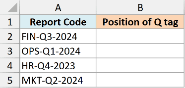
I want to find the position where the quarter tag starts, without knowing which quarter number it is.
Here is the formula:
=SEARCH("q?-", A2:A5)
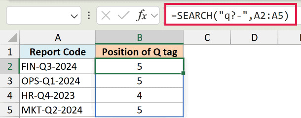
The question mark (?) is a wildcard that stands for any single character. So q?- tells SEARCH to look for a “q”, followed by any one character, followed by a dash.
That matches Q3-, Q1-, Q4-, and Q2- in the codes, and SEARCH returns the position where each tag begins.
Pro Tip: The asterisk (*) matches any sequence of characters, so q*4 would match a “q” with anything before the number 4. To search for a literal ? or *, put a tilde (~) in front of it.
Example 4: Check If a Cell Contains Specific Text
This is one of the most useful things you can do with SEARCH.
Below is a dataset of support notes in column B. I want to flag every note that mentions a refund.
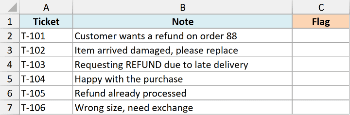
The problem is that SEARCH returns a position number when it finds the word, and a #VALUE! error when it doesn’t. I want a clean Flag instead.
Here is the formula:
=IF(ISNUMBER(SEARCH("refund", B2:B7)), "Flag", "")
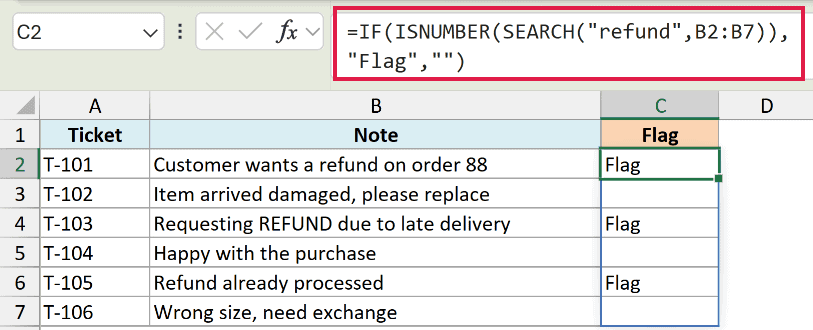
Here is how this formula works:
- SEARCH(“refund”, B2:B7) returns a number if “refund” is in the note, or a #VALUE! error if it is not.
- ISNUMBER turns that into TRUE (a number was returned) or FALSE (an error was returned).
- IF then shows “Flag” when the result is TRUE, and an empty string when it is FALSE.
Since SEARCH ignores case, the note that says “REFUND” in capitals gets flagged too.
This checks for matching text anywhere in the note, so “refunded” also gets flagged. It doesn’t check for a whole word.
Example 5: Extract Text with LEFT and SEARCH
Let’s use SEARCH to pull out part of a string.
Below is a dataset of names in column A, written as “Last, First”. I want to grab just the last name from each.
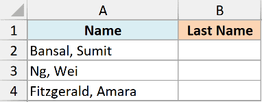
The last name is everything before the comma, so I need to know where the comma sits. That is where SEARCH comes in.
Here is the formula:
=LEFT(A2:A4, SEARCH(",", A2:A4)-1)
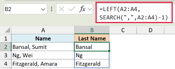
SEARCH finds the position of the comma in each name. I subtract 1 so I stop just before the comma, and LEFT pulls that many characters from the start of the string.
For “Fitzgerald, Amara”, the comma is at position 11, so LEFT returns the first 10 characters, which is “Fitzgerald”.
In Excel for Microsoft 365 or Excel 2024, TEXTBEFORE does this more directly:
=TEXTBEFORE(A2:A4,",")
The LEFT/SEARCH version above teaches how a found position becomes a character count. For older Excel, use a single-cell reference and fill the formula down.
Example 6: Extract Text Between Two Characters
Now let’s step it up with a more advanced use case.
Below are product codes in the format TRX-2024-BLU. I want to pull out the middle part (the year) that sits between the two dashes.
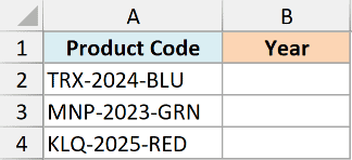
To do this, I need the position of both dashes. The trick is the third argument of SEARCH, which lets me start searching after the first dash.
Here is the formula:
=MID(A2, SEARCH("-",A2)+1, SEARCH("-",A2,SEARCH("-",A2)+1)-SEARCH("-",A2)-1)
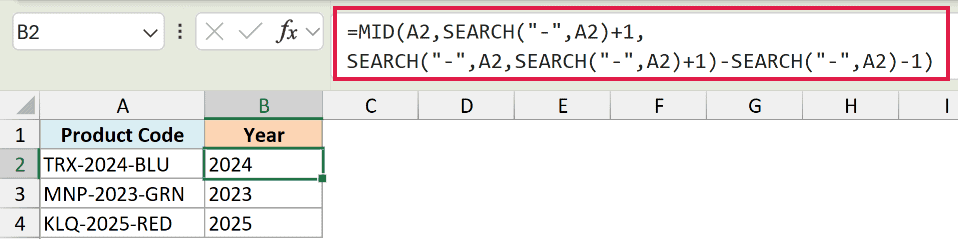
Here is how this formula works:
- SEARCH(“-“,A2) finds the first dash. Adding 1 gives me the position where the middle part begins.
- SEARCH(“-“,A2,SEARCH(“-“,A2)+1) starts searching one character after the first dash, so it finds the second dash.
- The difference between the two dash positions (minus 1) gives the length of the middle part, which MID then extracts.
For TRX-2024-BLU, this returns “2024”.
In Excel for Microsoft 365 or Excel 2024, this delimiter formula is simpler:
=TEXTBEFORE(TEXTAFTER(A2:A4,"-"),"-")
The MID/SEARCH version above teaches start_num and works in older Excel. Both methods expect two dashes in each code.
Example 7: Handle Not-Found Errors with IFERROR
Let’s finish with a way to keep your results clean.
Below is a dataset of order notes in column B. I want to find the position of the word “gift” in each note, but not every note has it.
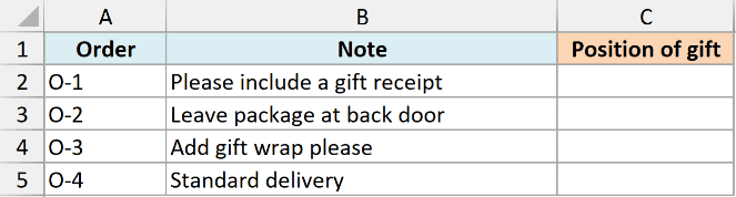
When SEARCH cannot find the word, it returns a #VALUE! error. Here is the plain formula so you can see the problem.
=SEARCH("gift", B2:B5)
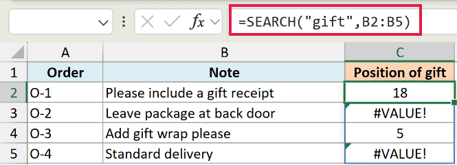
The notes that don’t mention a gift return #VALUE!, which looks messy. I can fix that by wrapping SEARCH in IFERROR.
Here is the improved formula:
=IFERROR(SEARCH("gift", B2:B5), "No gift note")
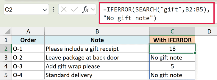
IFERROR checks the SEARCH result. If SEARCH finds the word, it shows the position. If SEARCH throws an error, IFERROR shows “No gift note” instead, so there are no ugly errors in your column.
IFERROR also hides errors already in the source cells, so “No gift note” doesn’t always mean the text was absent. Check unexpected results against the original notes.
Tips & Common Mistakes
- SEARCH is not case-sensitive. If you need an exact, case-sensitive match, use FIND instead. That is the main difference between the two functions.
- A #VALUE! error can mean missing text or an invalid start_num. start_num must be at least 1 and no greater than the text length. Wrap SEARCH in IFERROR to return a friendly message, or in ISNUMBER when you only need a TRUE/FALSE answer.
- Wildcards work in the find_text argument. Use
?for any single character and*for any sequence. To search for a literal?or*, type a tilde (~) before it. - Use the start_num argument to skip ahead. Passing a starting position lets you find the second (or later) occurrence of a character, which is handy for pulling text between delimiters.
- SEARCH counts spaces and punctuation. Every character in the string counts toward the position, including spaces, so the returned number reflects the true character position.
SEARCH is one of those small functions that quietly does a lot of heavy lifting. Once you get comfortable finding positions, you can combine it with LEFT, MID, IFERROR, and ISNUMBER to slice and check text in all sorts of ways.
Give these examples a try in your own sheet, and you’ll quickly see how often SEARCH comes in handy.
Other Excel Articles You May Also Like:
