

In this tutorial, you’ll learn how to find the position of the last occurrence of a character in a string in Excel.
A few days ago, a colleague came up with this problem.
He had a list of URLs, and he needed to extract all the characters after the last forward slash (“/”).
So for example, from https://example.com/archive/January he had to extract ‘January’.
It would have been really easy had there been only one forward slash in the URLs.
What he had was a huge list of thousands of URLs of varying length and a varying number of forward-slashes.
In such cases, the trick is to find the position of the last occurrence of the forward slash in the URL.
In this tutorial, I will show you three ways to find that position:
- Using the TEXTBEFORE function (Excel 365 and Excel 2024)
- Using a FIND and SUBSTITUTE formula (works in all versions)
- Using a custom function (created via VBA)
I’ll also show you how to find the last space in a text string, and how to use the position to extract the text after the last slash.
Follow along with the example file
Find Last Position of a Character in Excel.xlsm
Find the Last Occurrence of a Character Using TEXTBEFORE
If you’re using Excel 365 or Excel 2024, the TEXTBEFORE function gives you the shortest formula for this.
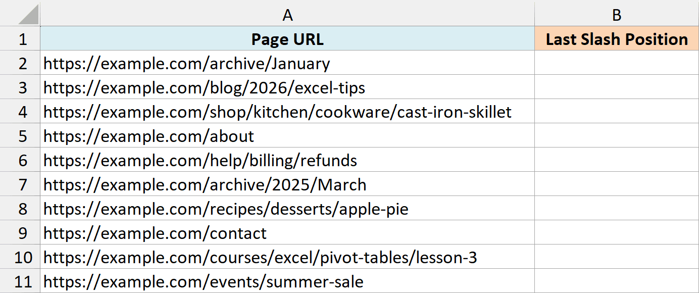
Below is a list of page URLs, and I want to get the position of the last forward slash in each URL in column B.
Here is the formula that will do this:
=LEN(TEXTBEFORE(A2:A11,"/",-1))+1
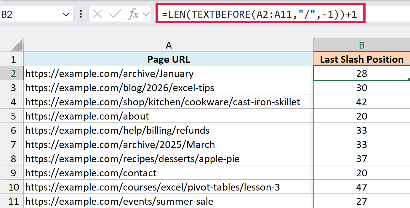
How this formula works:
- TEXTBEFORE(A2:A11,”/”,-1) – The -1 tells TEXTBEFORE to start looking from the end of the text, so it returns everything before the last forward slash. For the first URL, that’s https://example.com/archive.
- LEN(TEXTBEFORE(A2:A11,”/”,-1)) – This counts the characters in that text. For the first URL, it’s 27.
- +1 – The last forward slash comes right after that text, so adding 1 gives its position, which is 28.
You only need to enter this formula in cell B2. It spills down automatically and gives the position for every URL, so there’s nothing to copy.
If a cell has no forward slash at all, the formula returns #N/A. That’s useful, because it tells you the character isn’t in the text.
The TEXTBEFORE function is available in Excel 365 and Excel 2024. If you’re using an older version, the formula in the next section works everywhere.
Find a Character From the Right Using FIND and SUBSTITUTE
The FIND and SEARCH functions only look from left to right, so in older versions of Excel, we need a small trick that combines the FIND, SUBSTITUTE, and LEN functions.
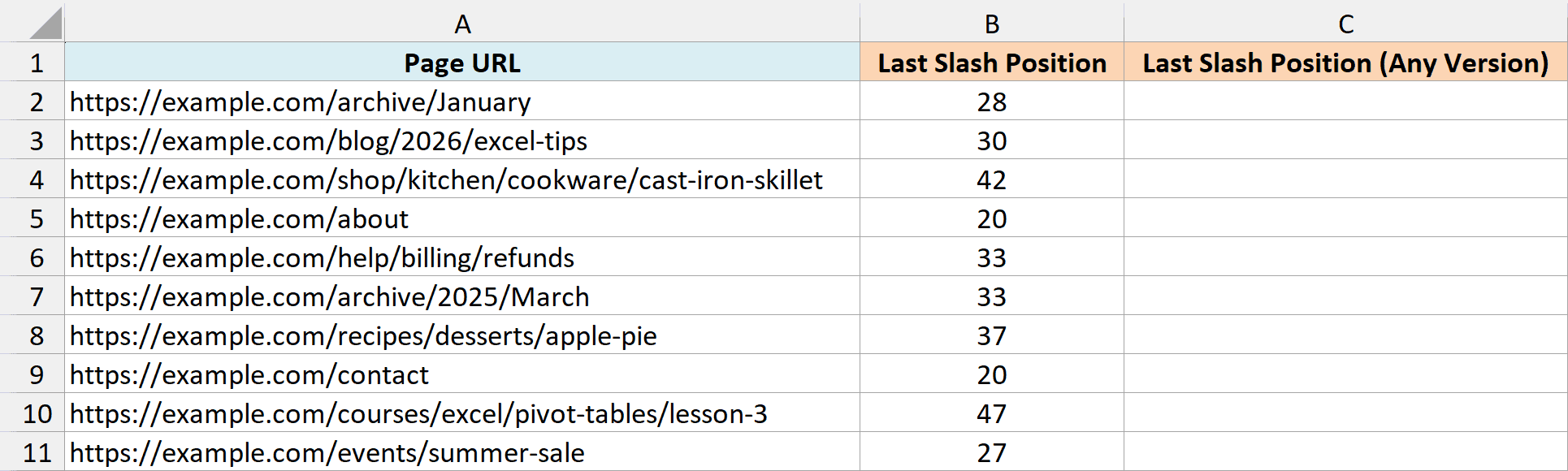
Below is the same list of page URLs with the TEXTBEFORE results in column B, and I want to get the position of the last forward slash with this formula in column C.
Here is the formula that will find the position of the last forward slash:
=FIND("@",SUBSTITUTE(A2,"/","@",LEN(A2)-LEN(SUBSTITUTE(A2,"/",""))))
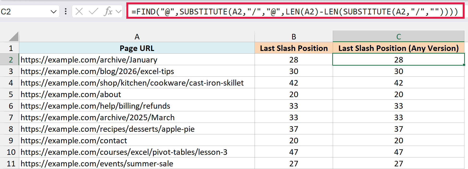
Enter this formula in cell C2 and copy it down for the rest of the URLs.
Let’s break down the formula and explain how each part of it works.
- SUBSTITUTE(A2,”/”,””) – This part of the formula replaces the forward slash with an empty string. In case you want to find the occurrence of any string other than the forward slash, use that here (and in the other places where the formula has “/”).
- LEN(A2)-LEN(SUBSTITUTE(A2,”/”,””)) – This part would tell you how many forward slashes are there in the string. It simply subtracts the length of the string without the forward slash from the length of the string with forward-slashes.
- SUBSTITUTE(A2,”/”,”@”,LEN(A2)-LEN(SUBSTITUTE(A2,”/”,””))) – This part of the formula would replace the last forward slash with @. The idea is to make that character unique. You can use any character you want. Just make sure it’s unique and doesn’t appear in the string already. The last argument of SUBSTITUTE tells it which occurrence to replace, so giving it the slash count (4 for the first URL) makes it replace the last one.
- FIND(“@”,SUBSTITUTE(A2,”/”,”@”,LEN(A2)-LEN(SUBSTITUTE(A2,”/”,””)))) – This part of the formula would give you the position of the last forward slash.
Important: If your text already has an @ before the last slash, FIND stops at that @ and gives you the wrong position. For https://medium.com/@name/post, it returns 20 instead of 25, so swap @ for a character like ~ that your data doesn’t have.
The slash count works because a forward slash is one character long. If you’re looking for a string with more than one character, such as “–“, divide the count by the length of that string.
Without that, the count comes out too big, and the formula returns #VALUE!. Here is the version for “–“:
=FIND("@",SUBSTITUTE(A2,"--","@",(LEN(A2)-LEN(SUBSTITUTE(A2,"--","")))/LEN("--")))
The slash formula in column C also returns #VALUE! when a cell has no forward slash at all, because the slash count is 0 and SUBSTITUTE has no 0th slash to replace.
Find the Last Space in a Text String
The same formulas work for any character, and one you’ll probably need often is the space character.
Below is a list of product names, and I want to get the position of the last space in each name in column B.
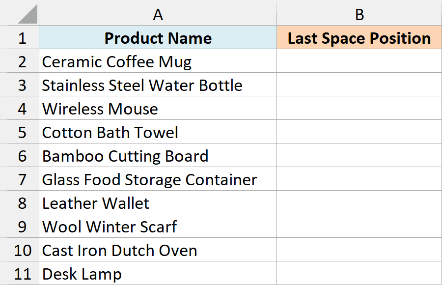
Here is the formula that will do this:
=LEN(TEXTBEFORE(A2:A11," ",-1))+1
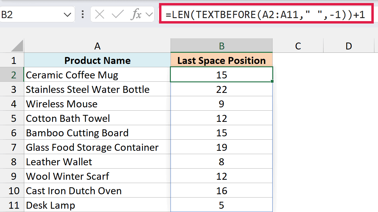
This is the same TEXTBEFORE formula from the first section, with a space (” “) in place of the forward slash. For Ceramic Coffee Mug, it returns 15, which is the space right before Mug.
If you’re using Excel 2021 or earlier, enter the below formula in cell B2 and then copy it down the range:
=FIND("@",SUBSTITUTE(A2," ","@",LEN(A2)-LEN(SUBSTITUTE(A2," ",""))))
A common reason to find the last space is to pull out the last word. If that’s what you’re after, the TEXTAFTER function (Excel 365 and Excel 2024) does it directly with =TEXTAFTER(A2:A11,” “,-1).
For names, see how to extract the last name in Excel.
Extract Text After the Last Occurrence of a Character
Now let’s go back to my colleague’s problem, which was to get everything after the last forward slash.
Below is the same list of page URLs, and I want to get the text after the last forward slash in each URL in column B.
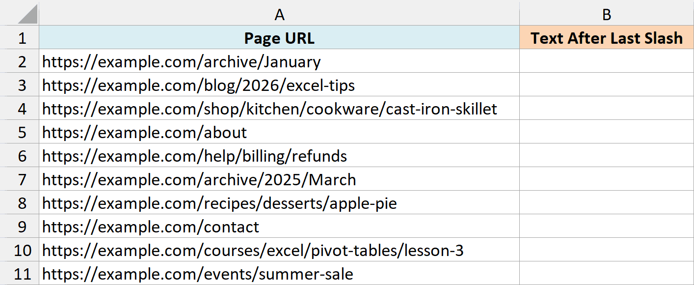
If you’re using Excel 365 or Excel 2024, the TEXTAFTER function pulls out this text in one step, without finding the position first. Here is the formula that will do this:
=TEXTAFTER(A2:A11,"/",-1)
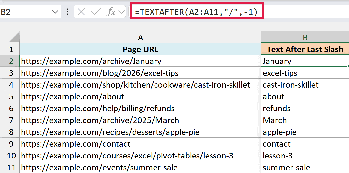
Just like TEXTBEFORE, the -1 makes TEXTAFTER start from the end, so it returns the text after the last forward slash. The formula spills down on its own, so you only enter it in cell B2.
Note that if a URL ends with a forward slash (like https://example.com/archive/), TEXTAFTER returns an empty cell, because nothing comes after the last slash.
In Excel 2021 or earlier, you need the position. When you have the position of the last occurrence, you can simply extract anything on the right of it using the RIGHT function.
Here is the formula that would find the last position of a forward slash and extract all the text to the right of it. Enter it in cell C2 and copy it down:
=RIGHT(A2,LEN(A2)-FIND("@",SUBSTITUTE(A2,"/","@",LEN(A2)-LEN(SUBSTITUTE(A2,"/",""))),1))
The FIND part is the same position formula from the earlier section (the 1 at the end tells FIND to start from the first character, which it does anyway). Here is what the rest does:
- LEN(A2)-FIND(“@”,SUBSTITUTE(A2,”/”,”@”,LEN(A2)-LEN(SUBSTITUTE(A2,”/”,””))),1) – This part of the formula would tell us how many characters are there after the last forward slash.
- =RIGHT(A2,LEN(A2)-FIND(“@”,SUBSTITUTE(A2,”/”,”@”,LEN(A2)-LEN(SUBSTITUTE(A2,”/”,””))),1)) – Now this would simply give us the string after the last forward slash.
Also read: Remove Last Character in Excel
Getting the Last Position of a Character using Custom Function (VBA)
While the FIND and SUBSTITUTE formula above is great and works like a charm, it’s a bit complicated.
If you’re comfortable using VBA, you can use a custom function (also called a User Defined Function) created via VBA. This can simplify the formula and can save time if you have to do this often.
For this case, I have created a function called LastPosition, that finds the last position of the specified character (which is a forward slash in this case).
Here is the VBA code that created this function:
Function LastPosition(rCell As Range, rChar As String) As Long
'This function gives the last position of the specified character
'This code has been developed by Sumit Bansal (https://trumpexcel.com)
LastPosition = InStrRev(rCell.Value, rChar)
End FunctionThe code uses VBA’s InStrRev function, which searches a string from the end and returns the position of the last match. If the character isn’t in the cell, it returns 0.
If you used the older version of this code from this page, replace it with the one above.
The old code returned one more than the actual position, showed #VALUE! when the character wasn’t in the cell, and missed a slash at the very end of the text.
To make this function work, you need to place it in the VB Editor. Once done, you can use this function like any other regular Excel function.
Here are the steps to place this code in the VB Editor:
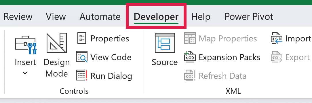
- Go to the Developer tab.
- Click on the Visual Basic option. This will open the VB editor in the backend.
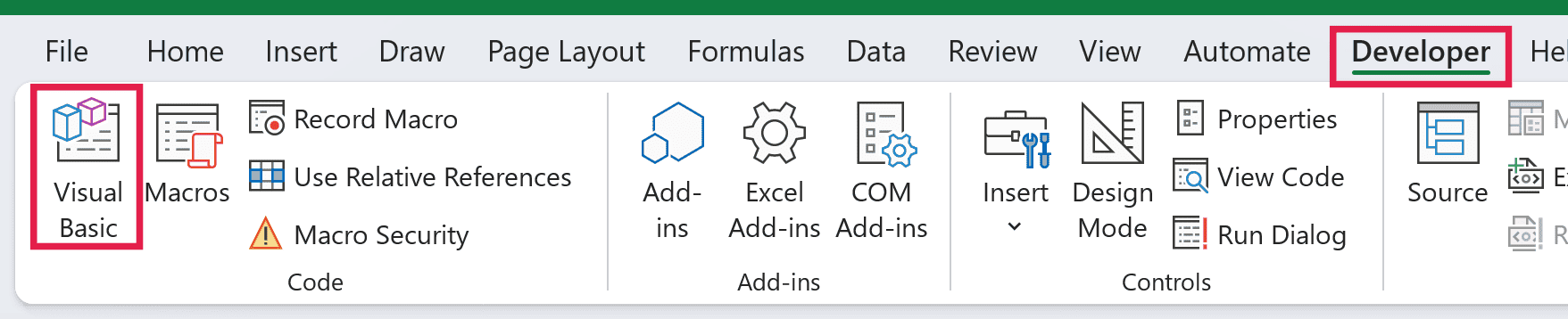
You can also press ALT + F11 to open the VB Editor, which is handy if you don’t see the Developer tab.
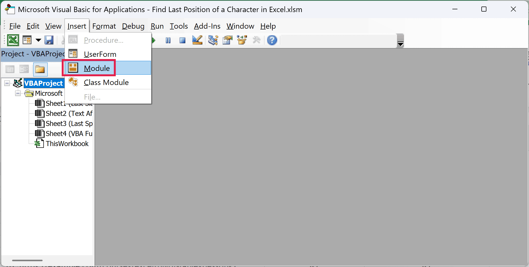
- In the Project Explorer pane in the VB Editor, right-click on any object for the workbook in which you want to insert the code. If you don’t see the Project Explorer go to the View tab and click on Project Explorer.
- Go to Insert and click on Module. This will insert a module object for your workbook.
- Copy and paste the code in the module window.
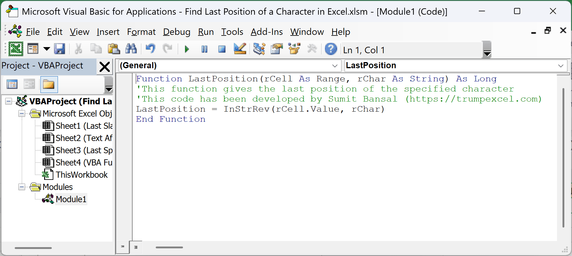
Now the LastPosition function would be available in all the worksheets of the workbook.
Let’s use the same data set of URLs, and get the position of the last forward slash in column B and the text after it in column C.
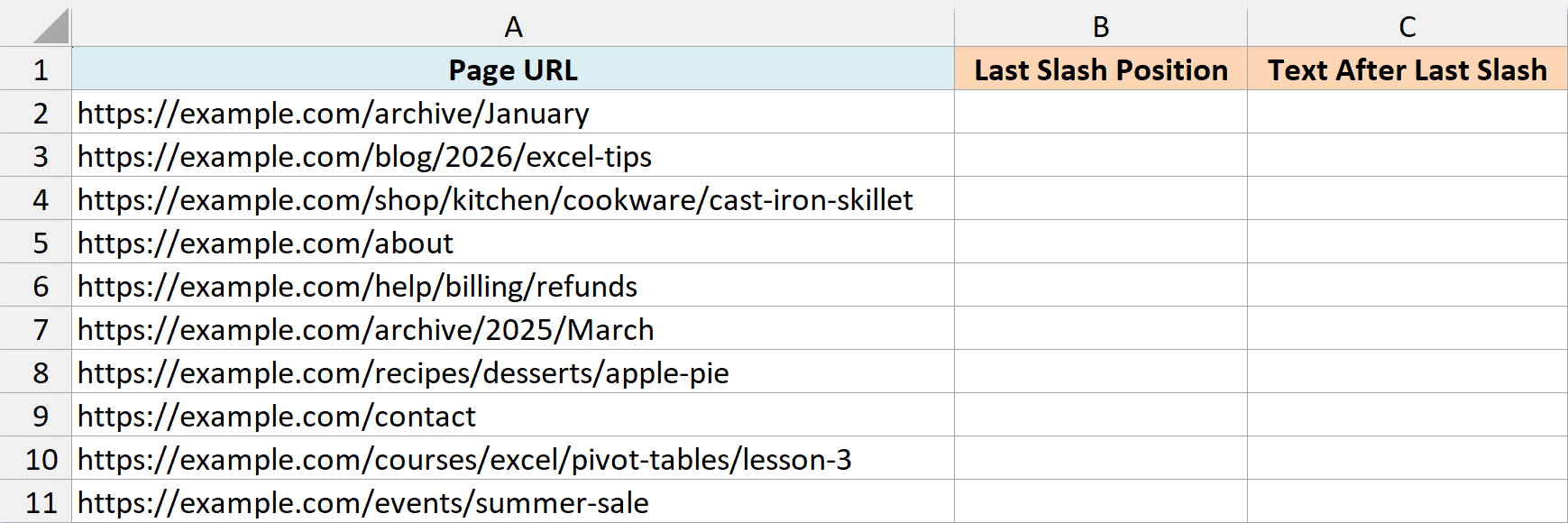
Here is the formula that gives the position of the last forward slash:
=LastPosition(A2,"/")
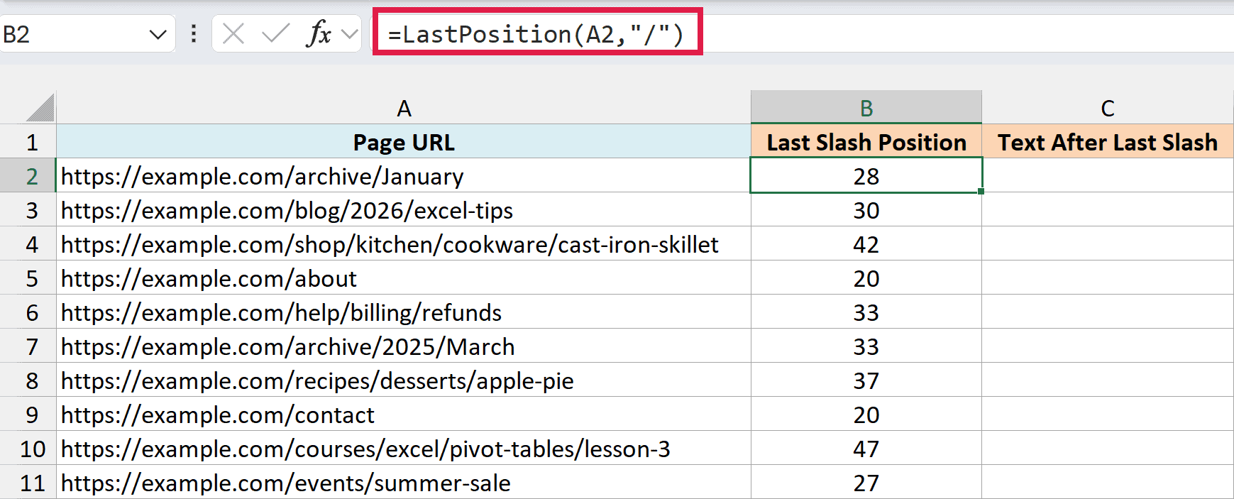
LastPosition – which is our custom function – returns the position of the forward-slash. This function takes two arguments – the cell reference that has the URL and the character whose position we need to find.
Enter it in cell B2 and copy it down. It gives the same positions as the formulas above, 28 for the first URL.
And here is the formula that will extract the text after the last forward slash:
=RIGHT(A2,LEN(A2)-LastPosition(A2,"/"))
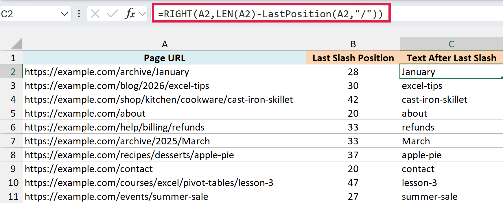
You can see that this is a lot simpler than the RIGHT and FIND formula we used above.
Here is how this works:
- LastPosition returns the position of the last forward slash, which is 28 for the first URL.
- LEN(A2)-LastPosition(A2,”/”) gives the number of characters after that slash.
- RIGHT function then gives us all the characters after the forward slash.
If a cell has no forward slash, LastPosition returns 0, so this formula returns the whole text.
The first argument has to be a cell reference, so LastPosition won’t work on text you type into the formula or on the result of another formula.
Note that you need to save the workbook as the .XLSM format as it has a macro in it.
Also, if you want this formula to be available in all the workbooks you use, you can either save it in the Personal Macro Workbook or create an add-in from it.
If you downloaded the example file and Excel blocks its macros, close the file, right-click it, and select Properties. Check Unblock on the General tab, click OK, and open the file again.
VBA doesn’t run in Excel for the web, so you need the desktop version of Excel for this method.
So these are three ways you can use to find the position of the last occurrence of a character in a string in Excel, and then use it to extract the text after it.
I hope you found this tutorial useful.
You May Also Like the Following Excel Tutorials:

Here is the non-VBA using LET
=LET(
Rmv_F_Slash, SUBSTITUTE($B10,””,””),
Num_F_Slash, LEN($B10)-LEN(Rmv_F_Slash),
Rplc_Last, SUBSTITUTE($B10,””,”@”,Num_F_Slash),
Psntn_Last, FIND(“@”,Rplc_Last),
Num_Chr_Aftr, LEN($B10)-Psntn_Last,
Full_Formula, RIGHT($B10, Num_Chr_Aftr),
Result, Full_Formula,
Result)
thank you
If you are searching for more than one character, for example “5.)”, in place of “/” in the equation example above, be sure to divide the length subtraction by the number of characters. This is because for every instance of that character string, that many characters are being removed from the string per instance, so the length subtraction equation gives you a difference that is *length of desired character string* greater than the number of instances.
E.g.,
=RIGHT(A2,LEN(A2)-FIND(“@”,SUBSTITUTE(A2,”/”,”@”,LEN(A2)-LEN(SUBSTITUTE(A2,”/”,””))),1)) [original]
=RIGHT(A2,LEN(A2)-FIND(“@”,SUBSTITUTE(A2,”5.)”,”@”,(LEN(A2)-LEN(SUBSTITUTE(A2,”5.)”,””)))/3),1)) [new]
Perfect! Thank you so much!! Saved me a lot of time:)
thank you
Thank you – used the cell formula and it worked a treat !
Or Excel specific:
InStrRev(rCell, rChar) + 1
Is the LastPosition() function not replaceable with…
InStrRev(MyString, “/”) + 1
?
I am so grateful. I was very hungry to get the formula. It will save a hundred hours of mine.
Works great! Thanks!
You guys just saved me a bunch of time – thank you!
Need help on formula to reverse the above process in reverse way,
Example:
Input: ABC123BCDSample.txt
Expected output: ABC123BCD
Using the example above, I used =MID(A2, 1, FIND(“@”,SUBSTITUTE(A2,”/”,”@”,LEN(A2)-LEN(SUBSTITUTE(A2,”/”,””))),1)-1)
You can remove “-1” if you want to include the last / in the output
This will remove everything after the final / in A1. Put this in in B1:
=SUBSTITUTE(A1,TRIM(LEFT(RIGHT(SUBSTITUTE(A1,”/”,REPT(” “,100)),100),100)),””)
Love it! Worked quick and easy !
Great explanation. Well Done and Thank you.
Thank you for this formula, this has saved me so much time today!
Excellent – thanks!
thanks for this, works great
sorry, doesn’t work
It does work you dummy, if you change the cell addresses correctly
Thanks so much for this — very helpful!
Worked great for me! Thank you!
The Excel formula is clever. But the VBA solution can be simplified by using the InStrRev function.
Works pretty well, but breaks if there’s only one of the separator character (“/”) in the string.