

If you want to swap out characters in a text string based on where they sit (say, the first four characters or the three characters starting at position five), the REPLACE function is what you’re looking for.
REPLACE works by position. You tell it where to start and how many characters to swap, and it drops in your new text. This is different from SUBSTITUTE, which finds and replaces matching text instead.
In Excel 365, you can also feed REPLACE a range and the results spill into the cells below. In this article, I’ll show you how to use REPLACE with six practical examples.
Follow along with the example file
REPLACE Function Examples.xlsx
REPLACE Function Syntax
Here is the syntax of the REPLACE function:
=REPLACE(old_text, start_num, num_chars, new_text)
- old_text – The original text (or the cell holding it) where you want to swap some characters.
- start_num – The position of the first character you want to replace. This must be at least 1.
- num_chars – How many characters, starting at start_num, you want to replace. This must be 0 or greater. Set this to 0 to insert text without removing anything.
- new_text – The text you want to drop in.
When to Use REPLACE in Excel
Use the REPLACE function when you need to:
- Swap characters at a known position, like a fixed prefix or a middle segment of a code.
- Mask sensitive data such as card or account numbers while keeping part of them visible.
- Insert a character (a dash, a space) into a string without deleting anything.
- Update a fixed part of many entries at once, like an area code or a year.
Let me show you a few practical examples of how this works.
Example 1: Replace Characters at a Fixed Position
Let’s start with a simple example.
Below is a dataset with order IDs in column A. Each ID starts with a four-digit year, followed by a dash and a sequence number.
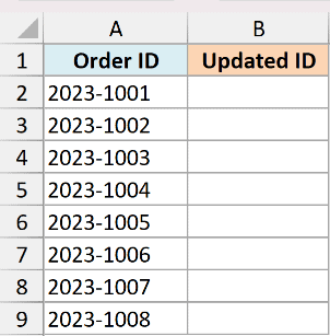
I want to update the year at the start of every ID from 2023 to 2024, leaving the rest of each ID untouched.
Here is the formula:
=REPLACE(A2:A9, 1, 4, "2024")
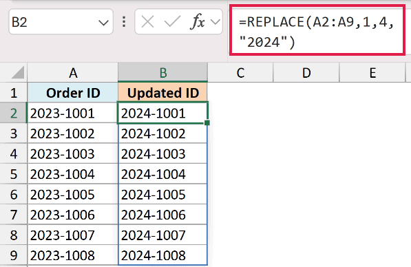
The formula starts at position 1, replaces the first 4 characters (the old year) with “2024”, and keeps everything from the dash onward. The same position-1 trick lets you remove the first character from a string by replacing it with a blank.
Since this is Excel 365, feeding REPLACE the whole range A2:A9 spills the results down the column in one go. No need to drag the formula down.
Pro Tip: If you’re on Excel 2019 or earlier, write the formula for the first cell as =REPLACE(A2, 1, 4, “2024”) and copy it down the column.
Example 2: Mask All But the Last 4 Digits of a Card Number
Here’s a scenario you’ll run into with sensitive data.
Below is a dataset with 16-digit card numbers stored as text in column A. Each one is a full number you don’t want on display.
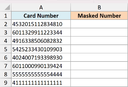
I want to hide the first 12 digits behind asterisks and show only the last 4 in the report.
The formula keeps the original numbers in column A. Before sharing, copy only the masked values into a separate report that doesn’t contain the original data.
Here is the formula:
=REPLACE(A2:A9, 1, 12, REPT("*", 12))
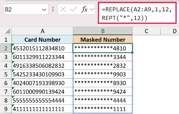
Here, REPLACE swaps the first 12 characters with a block of asterisks, and the last 4 digits stay in place. The REPT("*", 12) part just builds a string of 12 asterisks so I don’t have to type them out.
This works because every card number is exactly 16 characters. For different lengths, you need to adjust both the replacement count and the number of asterisks.
Pro Tip: Store card and account numbers as text before entering or importing them. Excel drops leading zeros and keeps only 15 significant digits when it stores numbers.
For 16-digit card numbers, digits beyond that limit are changed to zero. Formatting them as text afterward won’t restore the original digits.
Example 3: Insert Characters Without Deleting Any
This example uses a handy trick: setting num_chars to 0.
Below is a dataset with tracking codes in column A. They arrived as one solid block of characters, and I want to make them easier to read.
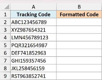
I want to insert a dash after the first three characters of each code, without removing any of the existing characters.
Here is the formula:
=REPLACE(A2:A9, 4, 0, "-")
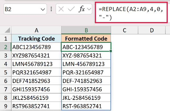
The key here is the 0 for num_chars. It tells REPLACE to replace nothing, so instead of swapping characters it simply inserts the dash at position 4 and pushes the rest of the string to the right.
This is the one thing SUBSTITUTE can’t do cleanly, since it needs existing text to match before it can put something in its place.
Example 4: Update an Area Code in Phone Numbers
Now let’s look at a case where the text you’re changing isn’t at the very start.
Below is a dataset with phone numbers in column A, written in the (212) 555-0189 format. The area code sits inside the parentheses.
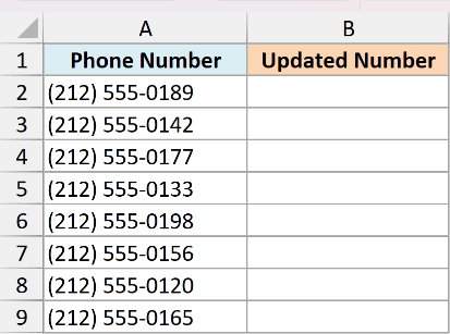
I want to update the area code from 212 to 646 across the list, while leaving the parentheses and the rest of each number as they are.
Here is the formula:
=REPLACE(A2:A9, 2, 3, "646")
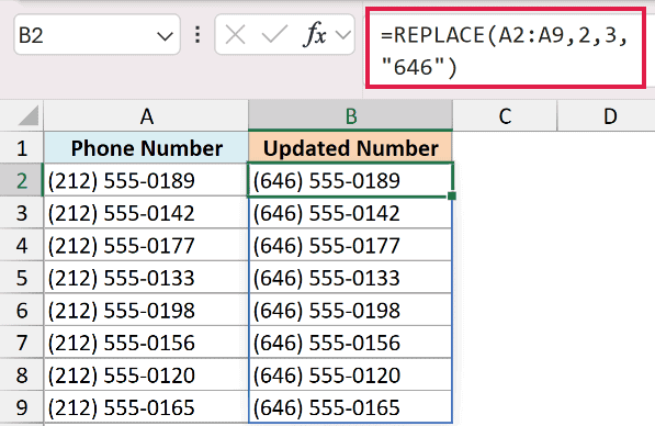
The area code starts at position 2 (right after the opening parenthesis) and is 3 characters long. So I start at 2, replace 3 characters, and drop in the new code.
This is where REPLACE really earns its keep. Because it works by position, it doesn’t matter that “212” might also appear elsewhere in the number. Only the three characters at position 2 get changed.
Example 5: Replace Text at a Dynamic Position with FIND
Let’s step it up with a more useful, real-world case.
Below is a dataset with email addresses in column A. The company rebranded, and every address needs to move from the old domain to the new one.
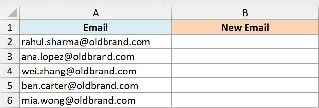
I want to swap the domain part (everything from the @ sign onward) to “@newbrand.com”. The catch is that the @ sits in a different position in every address, since the names have different lengths.
Here is the formula:
=REPLACE(A2, FIND("@", A2), LEN(A2) - FIND("@", A2) + 1, "@newbrand.com")
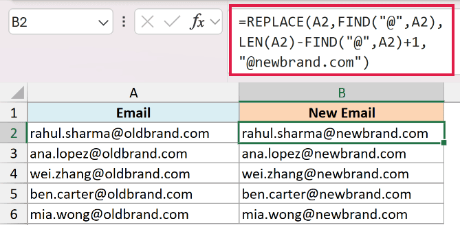
How this formula works:
- FIND(“@”, A2) locates the position of the @ sign, which becomes the dynamic start_num.
- LEN(A2) – FIND(“@”, A2) + 1 counts how many characters run from the @ to the end of the address, so REPLACE knows how much to swap.
- “@newbrand.com” is the new domain that gets dropped in.
By calculating the start position with FIND instead of hard-coding a number, the formula adjusts to each address on its own. This is the same idea you’d use to remove text before or after a specific character.
It’s a pattern to reach for whenever the thing you’re replacing doesn’t sit at a fixed spot. If you want to pull out part of a string instead of swapping it, see how to extract a substring with text formulas.
This example teaches how REPLACE uses a position found by FIND. For routine domain changes in Microsoft 365 or Excel 2024, extracting the username with TEXTBEFORE and adding the new domain is simpler.
Example 6: REPLACE vs SUBSTITUTE (Which One to Use)
This last one clears up the most common mix-up, so let’s compare the two side by side.
Below is a dataset with item codes in column A. Each code is department-year-department, and the same two-digit department number appears at both the start and the end.
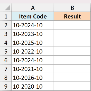
I want to change only the leading department number from 10 to 20, and leave the one at the end alone.
Here is the REPLACE formula:
=REPLACE(A2:A9, 1, 2, "20")
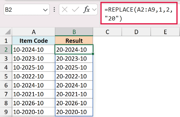
REPLACE works on position, so it only touches the two characters at the start and ignores the identical “10” at the end. The result is exactly what I wanted.
Now here is what happens if you try the same thing with SUBSTITUTE:
=SUBSTITUTE(A2:A9, "10", "20")
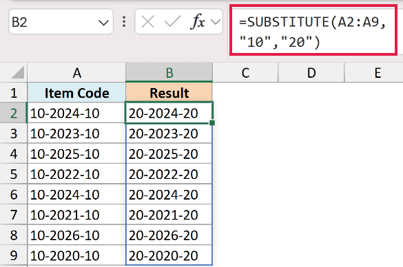
SUBSTITUTE matches text, not position, so it swaps every “10” it finds, including the one at the end. That gives you “20-2024-20”, which isn’t what you asked for.
The rule of thumb: use REPLACE when you know the position of what you’re changing, and use SUBSTITUTE when you know the text but not where it sits.
Tips & Common Mistakes
- REPLACE always returns text. Even if you replace characters in a number, the result comes back as a text string. Wrap it in VALUE if you need a number for further math.
- start_num begins at 1, not 0. The first character in a string is position 1. Setting start_num to 0 returns a #VALUE! error.
- Set num_chars to 0 to insert. This is the trick for adding a dash, space, or prefix without deleting anything (see Example 3).
- Invalid start_num or num_chars values cause a #VALUE! error. start_num must be at least 1 and num_chars at least 0. Numeric text such as “1” is accepted if Excel can convert it to a number.
- REPLACE by position, SUBSTITUTE by match. If the characters you want to change can appear more than once in the string, REPLACE targets the exact spot while SUBSTITUTE hits every occurrence unless you specify instance_num.
The REPLACE function is a simple but handy tool once you think about text by position. Whether you’re masking numbers, inserting separators, or updating a fixed prefix, it gives you precise control over exactly which characters change.
Pair it with FIND or LEN when the position isn’t fixed, and reach for SUBSTITUTE instead whenever you’re matching text rather than counting characters.
Other Excel Articles You May Also Like:
