

If you want to check whether any one of several conditions is true, the OR function is what you are looking for. It returns TRUE when at least one condition passes, and FALSE only when they all fail.
OR returns a single TRUE or FALSE, but it also works inside dynamic array formulas, which you will see in the last example.
In this article, I will walk you through the OR function with practical examples, from a simple two-condition check to pairing it with IF and AND.
Follow along with the example file
OR Function Examples.xlsx
OR Function Syntax
Here is the syntax of the OR function:
=OR(logical1, [logical2], ...)
- logical1 – The first condition you want to test. It has to evaluate to either TRUE or FALSE.
- logical2, … – Optional. Any additional conditions you want to test, up to 255 in total.
The function returns TRUE if any single condition is TRUE, and FALSE only when every condition is FALSE.
OR works in Excel for Microsoft 365, Excel 2024, 2021, 2019, and 2016, as well as Excel on the web.
Pro Tip: OR is inclusive, so it returns TRUE if one, some, or all of your conditions are true. With two conditions, XOR returns TRUE when exactly one is true. With more conditions, XOR tests whether an odd number are true.
When to Use the OR Function
Reach for the OR function when you need to:
- Check if a row meets at least one of several conditions
- Flag records that match any value from a short list
- Feed a single TRUE or FALSE into an IF formula so it acts when any condition holds
- Build a conditional formatting rule that lights up on any of several triggers
Let me show you a few practical examples of how the OR function works.
Example 1: OR With Multiple Conditions
Let’s start with a simple example.
Below is a small table of support tickets. Column A has the ticket ID, column B has the priority, and column C has the customer tier.
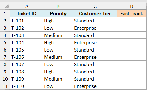
I want to flag a ticket for fast-track handling if its priority is High or the customer is on the Enterprise tier.
Here is the formula:
=OR(B2="High",C2="Enterprise")
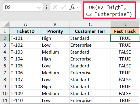
Here, OR checks two conditions. If the priority in B2 is High, or the tier in C2 is Enterprise, it returns TRUE. If neither is true, it returns FALSE.
Only one of the two conditions needs to be true for the result to be TRUE. That is the whole idea behind OR.
Since both conditions compare against text, High and Enterprise are wrapped in double quotes.
Example 2: OR With Comparison Operators
Now let’s use OR with numbers instead of text.
Below is a fitness log. Column A has the date, column B has the step count for the day, and column C has the active minutes.
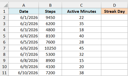
I want to mark a day as counting toward my streak if I hit at least 8,000 steps or at least 30 active minutes.
Here is the formula:
=OR(B2>=8000,C2>=30)
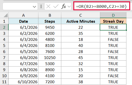
Each condition here uses a comparison operator. B2>=8000 checks the steps, and C2>=30 checks the active minutes.
If either one comes back TRUE, the whole formula is TRUE. So a low-step day still counts as long as the active minutes are there.
Unlike the text conditions in the first example, number comparisons like >=8000 don’t need any quotes around them.
Example 3: Using IF With the OR Function
OR really shines when you drop it inside an IF function.
On its own, OR only returns TRUE or FALSE. Pair it with IF and you can return any label or value you want instead.
Below is a field-trip tracker. Column A has the student name, column B shows whether the signed slip is in (Yes or No), and column C shows the payment status (Paid or Unpaid).
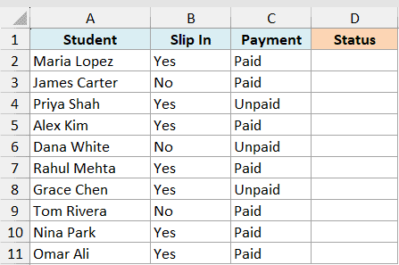
I want a column that says Follow Up when the slip is missing or the payment is still unpaid, and All Set otherwise.
Here is the formula:
=IF(OR(B2="No",C2="Unpaid"),"Follow Up","All Set")
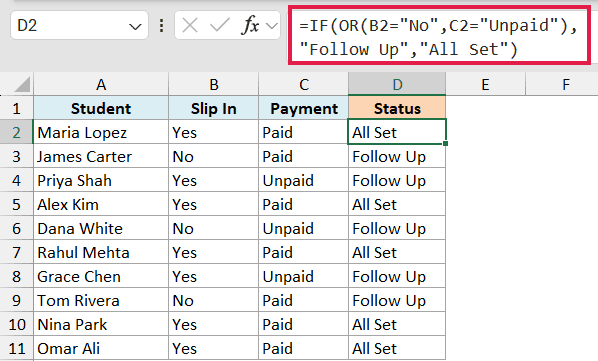
The OR sits in the logical test of IF. If the slip is No, or the payment is Unpaid, OR returns TRUE and IF shows Follow Up.
When both are fine (slip in and payment paid), OR returns FALSE and IF shows All Set.
Pro Tip: You can stack more conditions inside the same OR, like =IF(OR(B2=”No”,C2=”Unpaid”,E2=”No”),…) if you add a third check in column E. The IF still fires the moment any one of them is true.
Example 4: Combining OR and AND in One Formula
Let’s step it up and mix OR with AND.
Sometimes a rule needs both an either-or part and a must-be-true part. You can nest OR inside AND to handle that.
Below is a list of job applicants. Column A has the name, column B has years of experience, column C has the highest degree, and column D shows whether they hold a certification (Yes or No).
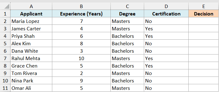
I want to shortlist an applicant for an interview only if they have at least 5 years of experience and they either hold a Masters degree or a certification.
Here is the formula:
=IF(AND(B2>=5,OR(C2="Masters",D2="Yes")),"Interview","Review")
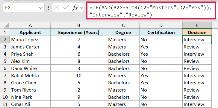
How this formula works:
- OR(C2=”Masters”,D2=”Yes”) returns TRUE if the applicant has a Masters degree or holds a certification.
- AND(B2>=5, …) then requires two things at once: at least 5 years of experience and that OR result being TRUE.
- IF shows Interview when the whole AND is TRUE, and Review otherwise.
So experience alone isn’t enough, and a qualification alone isn’t enough. The applicant needs the experience plus at least one of the two credentials.
Example 5: Flag Rows With OR Using a Dynamic Array
Here’s a modern approach that most people haven’t seen.
OR by itself gives you one TRUE or FALSE for one row. If you want to check every row in one go, you can wrap OR inside BYROW so the results spill down the column.
Below is a project status board. Column A has the project name, and columns B, C, and D each hold a Yes or No for On Track, On Budget, and Fully Staffed.
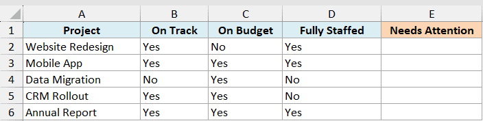
I want a single formula that flags TRUE for any project where at least one of those three checks is a No.
Here is the formula:
=BYROW(B2:D6,LAMBDA(row,OR(row="No")))
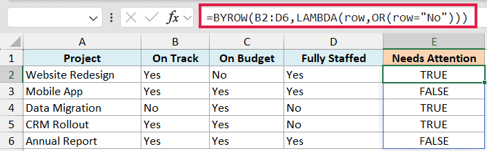
How this formula works:
- BYROW walks through B2:D6 one row at a time and hands each row to the LAMBDA.
- OR(row=”No”) checks that row’s three cells and returns TRUE if any of them is No.
- Because BYROW returns one result per row, the TRUE and FALSE values spill down the column from a single formula.
You type it once and all five projects in B2:D6 get flagged. If you add a project below row 6, extend B2:D6 in the formula to include that row.
Pro Tip: BYROW and LAMBDA are in Microsoft 365, Excel 2024, and Excel for the web. On Excel 2021 or earlier, put =OR(B2=”No”,C2=”No”,D2=”No”) in the first row and copy it down instead.
Tips & Common Mistakes
- OR returns just one value, even over a range. In Excel 2019 and earlier, confirm a range check like this with Ctrl+Shift+Enter. A formula like =OR(A2:A10>5) does not check each row separately. It scans the whole range and returns a single TRUE if any cell is greater than 5. For a per-row check, compare single cells or use the BYROW approach from Example 5.
- Text conditions need double quotes. =OR(B2=”High”,C2=”Low”) works, but leaving the quotes off makes Excel treat High and Low as names and throw an error.
- A #VALUE! error usually means no logical values. If you point OR at a range that holds only text or blanks with nothing to evaluate as TRUE or FALSE, it returns #VALUE!. Make sure at least one argument resolves to a logical value.
- Use + for OR logic inside FILTER. When you use the FILTER function, OR won’t split the conditions per row, because it collapses everything into a single TRUE or FALSE. Add them instead, like FILTER(data,(x=”A”)+(x=”B”)), where the + acts as OR.
- Need every condition true instead of any? Swap OR for the AND function, which only returns TRUE when all conditions pass.
The OR function is a small but handy tool once conditional logic enters your spreadsheets. Start with a couple of conditions, drop it inside IF when you need a label, and reach for BYROW when you want to check every row at once.
I hope you found this tutorial helpful. Let me know in the comments if you have any questions.
Other Excel Articles You May Also Like:
