

If you want to flip a logical test in Excel, so a TRUE becomes FALSE and a FALSE becomes TRUE, the NOT function is what you need.
It takes a single condition and reverses the result. That comes in handy when it’s easier to describe what you don’t want than what you do.
In Excel for Microsoft 365, Excel 2024, Excel 2021, and Excel for the web, you can also feed NOT a whole range and the results spill into the cells below.
In this article, I’ll show you how to use the NOT function with practical examples, from reversing a simple comparison to using it inside IF, OR, and data validation.
Follow along with the example file
NOT Function Examples.xlsx
NOT Function Syntax
Here is the syntax of the NOT function:
=NOT(logical)
- logical – the value or expression you want to reverse. It has to be something Excel can read as TRUE or FALSE, like a comparison (
A2>100), a logical value, or another function that returns TRUE or FALSE.
NOT takes exactly one argument. If you want to test several conditions at once, combine them with the AND function or OR first, then wrap the whole thing in NOT.
NOT works in Excel for Microsoft 365, Excel 2024, 2021, 2019, 2016, and Excel on the web, so you can use it just about anywhere.
When to Use the NOT Function
Use the NOT function when you need to:
- Reverse the result of a logical test, turning a TRUE into a FALSE
- Check that a condition is not met, like a cell that is not blank or a status that is not “Closed”
- Pair it with IF, AND, or OR to build a rule that’s easier to state as an exclusion
- Set up a data validation or conditional formatting rule that blocks certain entries
Let me show you a few practical examples of how this works.
Example 1: Reverse a Comparison with NOT
Let’s start with the simplest case: flipping the result of a comparison.
Below I have a small orders table, with the order ID in column A and the delivery status in column B. Each order is marked Delivered, Pending, or In Transit.
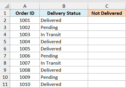
I want a TRUE for every order that has not been delivered yet, so I can see at a glance what still needs attention.
Here is the formula:
=NOT(B2:B11="Delivered")
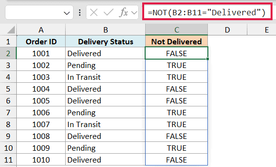
In the above formula, B2:B11="Delivered" first checks each status and returns TRUE for the delivered orders and FALSE for the rest. NOT then flips each result, so a delivered order becomes FALSE and everything else becomes TRUE.
Because I passed the whole range B2:B11 at once, the formula spills the TRUE/FALSE results down the column on its own. You type it once and Excel fills the rest.
Pro Tip: The spilling version needs Microsoft 365, Excel 2024, Excel 2021, or Excel for the web. On Excel 2019 or earlier, put =NOT(B2=”Delivered”) in the first cell and copy it down.
Example 2: Combine NOT with the IF Function
Now let’s turn that TRUE/FALSE into something more useful with the IF function.
Below I have a list of team members in column A and whether they finished the compliance training in column B, marked Yes or No.
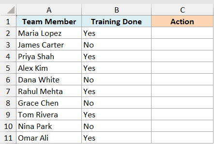
I want a reminder note next to anyone who has not completed the training, and a blank cell for those who have.
Here is the formula:
=IF(NOT(B2:B11="Yes"),"Send reminder","")
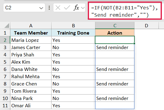
Here, NOT(B2:B11="Yes") is TRUE for every person whose status is not Yes. IF reads that result and returns “Send reminder” when it’s TRUE, or an empty string when it’s FALSE.
This reads the way you’d say it out loud: if the training is not done, send a reminder. Stating the condition as an exclusion is often clearer than listing every value that should pass.
Example 3: Check That a Cell Is Not Blank
A really common use of NOT is pairing it with ISBLANK to check whether a cell actually has something in it.
Below I have a list of survey invites in column A and the response each person left in column B. Some people replied, and some cells are still empty.
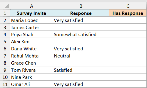
I want to mark which rows have a response recorded, so I can tell at a glance who has replied so far.
Here is the formula:
=NOT(ISBLANK(B2:B11))
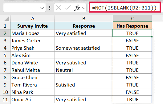
ISBLANK(B2:B11) returns TRUE for the empty cells and FALSE for the ones that hold a response. NOT flips that, so you get TRUE for nonempty cells and FALSE for empty ones.
A formula returning "" or a cell containing spaces is not empty.
This works well as a helper column. You can wrap it in an IF to show a status label, or use it as the test inside other formulas.
Example 4: Exclude Multiple Values with NOT and OR
You can also use NOT to knock out more than one value at once by teaming it up with the OR function.
Below I have a support log with the ticket ID in column A and its current status in column B (Open, Closed, Cancelled, or Escalated). Closed and Cancelled tickets are done, so I don’t need to see them.
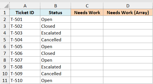
I want to flag every ticket that still needs work, meaning any status that is not Closed and not Cancelled.
Here is the formula:
=NOT(OR(B2="Closed",B2="Cancelled"))
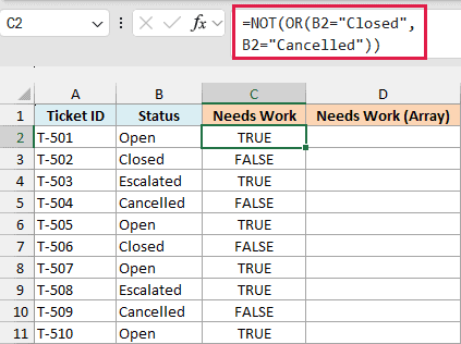
OR(B2="Closed",B2="Cancelled") returns TRUE when the status is either Closed or Cancelled. NOT reverses it, so the result is TRUE only when the ticket is neither of those, which is exactly the ones that still need attention.
I’m keeping this one as a per-row formula because OR collapses a range down to a single TRUE/FALSE. To flag the whole column in one go, use the array version instead:
=NOT((B2:B11="Closed")+(B2:B11="Cancelled"))
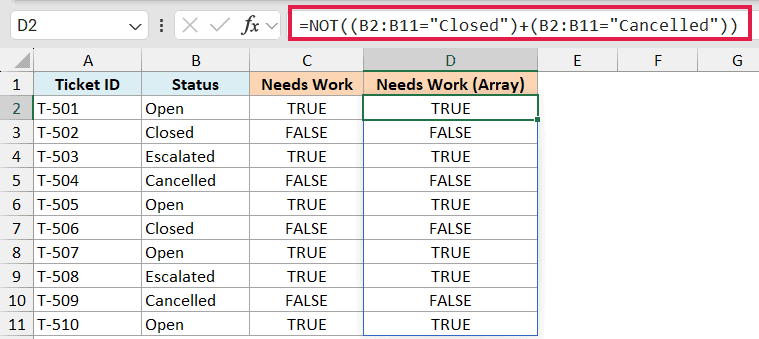
Here the two comparisons each produce a column of TRUE/FALSE values. Adding them with + acts like OR across the range, giving 1 where a ticket is Closed or Cancelled and 0 otherwise. NOT then flips that, so it spills a TRUE next to every ticket that still needs work.
Example 5: Use NOT in a Data Validation Rule
NOT is also useful inside data validation, where you want to block certain entries instead of just flagging them.
Say you have a booking sheet where people enter a delivery date in column A, and you want to stop anyone from choosing a Saturday or Sunday.
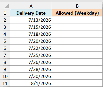
I want Excel to reject any weekend date the moment someone types it into column A.
Select the cells you want to protect, go to Data > Data Validation, choose Custom under Allow, and enter this formula:
=NOT(OR(WEEKDAY(A2)=1,WEEKDAY(A2)=7))
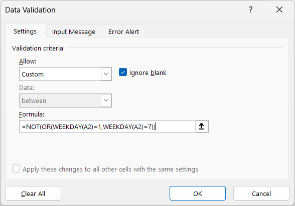
WEEKDAY returns 1 for Sunday and 7 for Saturday. So OR(WEEKDAY(A2)=1,WEEKDAY(A2)=7) is TRUE on a weekend, and NOT flips it to FALSE.
Data validation only accepts an entry when the formula returns TRUE, so weekday dates pass and weekend dates get rejected. Point the formula at the first cell of your selection (A2 here, since row 1 holds the header) and Excel applies the same logic to every cell.
Column B runs the same formula as a visible check, showing TRUE for weekdays and FALSE for weekends. Data validation only checks new entries as you type them, so the weekend dates already in column A stay there for column B to flag.
Pro Tip: The same formula works as a conditional formatting rule. Use it to shade weekday dates instead of blocking them.
Tips & Common Mistakes
- NOT takes exactly one argument. It reverses a single TRUE/FALSE value. To test several conditions, combine them with AND or OR first, then wrap the whole thing in NOT.
- NOT works on numbers too. Any non-zero number counts as TRUE, so NOT returns FALSE for it, and NOT(0) returns TRUE. That’s why the array trick in Example 4 works.
- For “not equal to”, you often don’t need NOT. A plain
<>comparison likeA2<>100is shorter thanNOT(A2=100)and does the same job. Reach for NOT when you’re reversing a function’s result, not a simple comparison. - Double negatives cancel out.
NOT(NOT(A2>5))is justA2>5. If you find yourself nesting NOTs, there’s usually a simpler way to write the condition. - The spilling form needs dynamic-array Excel. Feeding NOT a range spills in Microsoft 365, Excel 2024, Excel 2021, and Excel for the web. On Excel 2019 or earlier, enter the formula in the first cell and copy it down.
Wrapping Up
The NOT function is small, but it makes your logical formulas easier to read whenever the simplest way to describe a rule is to say what you don’t want. Once you start pairing it with IF, OR, and data validation, you’ll find plenty of places to use it.
I hope you found this tutorial helpful.
Other Excel Articles You May Also Like:
