
What comes to your mind when you see text with a strikethrough in Excel (something as shown below)?
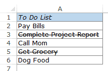
In most cases, it means that the task or activity has been completed and has been checked off.
Those who work with Microsoft Word use this extensively, and there is a strikethrough icon right there in the ribbon.
However, there is no icon in the Excel ribbon to do this.
In this tutorial, I will share various ways to access the strikethrough option and apply it to text in Excel.
Keyboard Shortcut to Apply Strikethrough in Excel
Here is the keyboard shortcut that will automatically apply the strikethrough formatting in Excel.
Control + 5
Just select the cell where you want to apply the strikethrough format and press Control + 5.
If you want to apply this to a range of cells, select the entire range of cells, and use this keyboard shortcut. You can also select non-adjacent ranges and then apply the strikethrough format.
See Also: 200+ Excel Keyboard Shortcuts.
Add Icon in QAT to Access Strikethrough in Excel
While the icon is not available in the ribbon or Quick Access Toolbar (QAT) by default, you can add it easily. Here are the steps to add strikethrough icon in the QAT:
- Right-click on any existing QAT icon or the ribbon tabs and select ‘Customize Quick Access Toolbar…’.
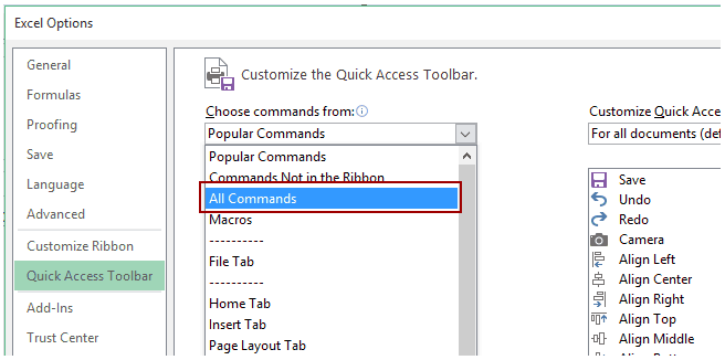
- In the Excel Options dialog box, select All Commands from the drop-down.
- Scroll down and select Strikethrough from the list. Click on Add.
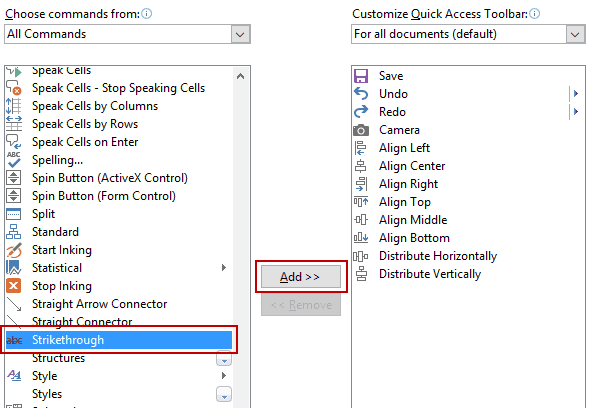
- Click OK. This will add the strikethrough icon in the quick access toolbar.
Also read: Filter Cells with Bold Font Formatting in Excel
Access Strikethrough Format from Format Cells Dialog Box
There is another way you can access strikethrough in Excel – Using the Format Cells dialog box.
While the earlier mentioned techniques (keyboard shortcut and icon) are faster ways to access strikethrough formatting, using the Format cells dialog box gives you access to a lot of other formatting options as well.
Here are the steps to access Strikethrough in Excel using the Format Cells dialog box:
- Select the cells where you want to apply the strikethrough format.
- Press Control + 1 (or right-click and select Format Cells).

- In the format cells dialog box, select the font tab and check the Strikethrough option.

- Click OK. This would apply the strikethrough format to the selected cells.
While this option is longer as compared to a keyboard shortcut or using the icon, it also gives access to many other formatting options in a single place. For example, you can also change color, font type, font size, border, number format, etc., using this dialog box.
Also read: Remove Strikethrough in Excel
Examples of Using Strikethrough in Excel
Strikethrough in Excel can be used to show completed tasks.
Here are three practical examples where you can use the strikethrough format in Excel.
EXAMPLE 1: Using Conditional Formatting
We can use conditional formatting to strikethrough a cell as soon as it is marked as completed.
Something as shown below:
See Also: How to create a drop-down list in Excel.

EXAMPLE 2: Using Checkboxes (to show completed tasks)
You can also use check-boxes to cross off items. Something as shown below:
EXAMPLE 3: Using Double Click (VBA)
If you are cool with using Excel VBA macros, you can also use the double-click event to cross off items simply by double-clicking on it. Something as shown below:
This method disables getting into the edit mode on double click and simply applies the strikethrough format as soon as you double click in the cell (VBA code available in the download file).
While the idea behind applying the strikethrough format in Excel remains the same, you can get as creative as you want.
Here is a creative example where I used the strikethrough format in a Task Prioritization Matrix template.
I hope you found this article useful. Let me know your thoughts in the comments section.
You May Also Like the Following Excel Tutorials:


sir its all usefull for me. i have improve my self along without completing any course
thank you to all special admin
It may sound odd, but I still use old school pen and paper(scrape paper) to write off my tasks in office. But many times the paper on which I had written my task gets misplaced, and with it all my plans for that day. I was procrastinating on using any new software to manage my simple to do list, but yours strikethrough has inspired me to use excel as my to do list instead of paper because I’m quite familiar with it, plus strikethrough will give me the satisfaction I get when I cross items off my list. 😀 Thanks for sharing it Sumit.
It is really a temptation to use strike-through to cross out records visually. However, we have to use it with caution in Excel. It is a good practice to accompany it with a remark, like what you did in Example 1.
Why am I saying that? Because we cannot filter records with strike-through. Think about if you are maintaining a table of more than 1000 records with hundreds of strike-through (that indicates completed job)… then one day your boss asks you a simple question: How many records have been completed???… Without a supplementary remark, it could be a nightmare to get the answer for a simple question.
Of course, there is a workaround, which requires a combination of simple techniques:
http://wmfexcel.com/2013/12/05/quickly-deletehide-records-rows-with-strikethrough-format-by-using-find-and-a-couple-of-simple-techniques/
but still a column with appropriate remarks is more handy and useful to majority of user. Isn’t is?
Hello Wong.. Thanks for commenting and sharing.
A good workaround to count/filter/hide the number of strike through cells would be to use find and replace and apply a color to it. That ways you can now filter/sort it using that color. This can also quickly answer ‘how many records have been completed?’
While it is a good option to have a complimentary column, I guess most the people would not create one while checking off items.