Repeat Rows N Times in Excel

If you want to repeat rows in your dataset N number of times (say 5 or 7 times), or based on a value in a column, Power Query is the easiest way to do that.

In this article, I’ll walk you through two methods to repeating all rows the same number of times, and repeating rows based on different values that are given in a column.

So let’s get to it!

1. Repeat All Cells / Rows N Times

Below I have a dataset of all-time top grossing movies as of writing this article. And I want to repeat each row in this data five times.

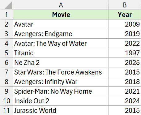
Note: While I’m going to show you how to repeat rows in a data set, you can use the same process to also repeat cells in a column

Here are the steps to do this using Power Query.

Step 1: Convert Your Data to an Excel Table

If your data is already in an Excel table, you can leave this step. But if it’s not, you can use the below steps to first convert you data into an Excel Table.

1. Select any cell within your data
2. Hold the Ctrl key and press the T key
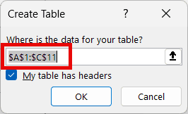
3. In the Create Table dialog box that opens, verify that range is correct (it usually is)
4. Ensure “My table has headers” is checked (if your data includes headers)

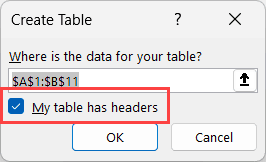
5. Click OK

Now your data has been converted into an Excel Table.

Optional: For the sake of simplicity and clarity, it best to rename your Excel Table and give it a descriptive name. In this case, I will name it RepeatRows

Step 2: Open Power Query

Now let’s open this table in Power Query Editor.

1. Select any cell in the Excel Table.
2. Go to the Data tab in the Excel ribbon and click on the “From Table/Range” icon

This will open your data in the Power Query Editor.

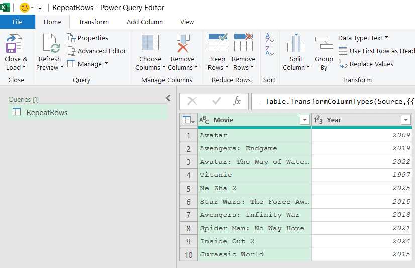
Note that the name of the query will be the same as the name of your table.

Step 3: Create a List Using a Custom Column

Now we will insert a new column that will be used in the next step to make the rows repeat.

To do this:

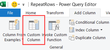
1. In the Power Query Editor, click the “Add Column” tab

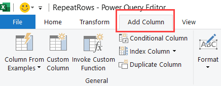
2. Click on “Custom Column” option

3. In the “New column name” field, enter any name you prefer. I will leave it as Custom
4. In the formula field, type: {1..5} (This creates a list of numbers from 1 to 5 and every cell in the newly added column will get this list)

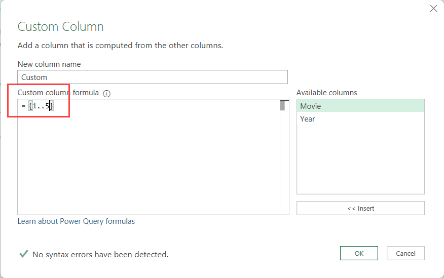
5. Click OK

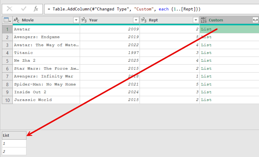
Once done, you will see that the new column displays a “List” value in each cell (as shown below).

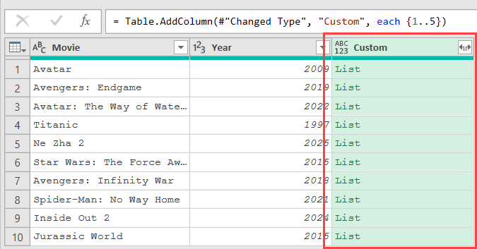
This might look strange if you’re new to Power Query! What’s happening is that Power Query has created a small container (called a list) for each row, and inside each container are five numbers: 1, 2, 3, 4, and 5.

If you click on any “List” value in this new column, you’ll see these numbers appear in the preview window at the bottom of your screen.

This is different from regular Excel where a cell typically holds just one value. In Power Query, a cell can hold multiple values in a list, which is exactly what we need to repeat our rows in the next step.

Step 4: Expand the List to Rows

Now that we have the list in each cell in the newly added column, let expand it so it gives the repeated rows.

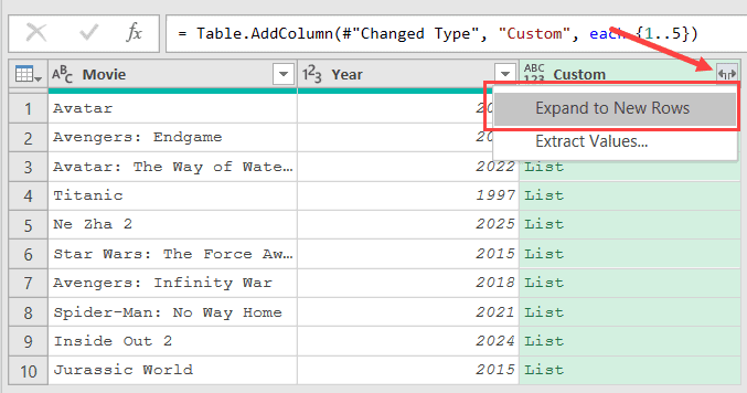
1. Click the expand icon (two diagonal arrows) on your new custom column
2. Select “Expand to New Rows”

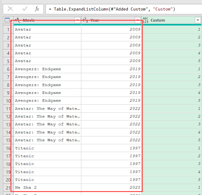
And Voila!

You can see we are very close to what we wanted. Every row in the dataset has been repeated five times.

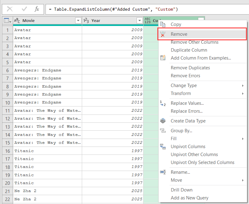
Step 5: Remove the Custom Column

Now let’s remove the column we inserted:

1. Right-click on the custom column header
2. Select “Remove”

As this point, we have the data we want, but it’s in Power Query editor. So we need to get this data into Excel now.

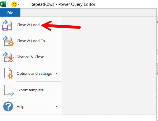
Step 6: Load the Data to Excel

1. Go to File tab
2. Click on Close & Load

This will insert a new sheet into your Excel workbook and the resulting data from Step 5 will be inserted as an Excel Table.

Power Query Magic: The real Power Query Magic happens when there are changes and you want to redo this result. Insetad of repeating all these steps again, just right click on any cell in the resulting table and click on Refresh. Since we have already created the query, all the steps would repeat in the backend and your results would be refreshed (almost instantly)

Also read: Create All Possible Combinations from Lists in Excel

2. Repeat All Cells / Rows Based on Different Values

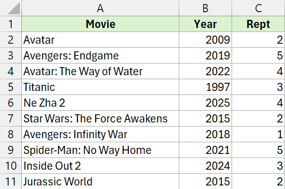
What if you don’t want to repeat each row the same number of times? Maybe you want the first row to repeat 2 times, the second row 5 times, the third row 4 times, and so on?

Below I have a dataset where I have a column named ‘Rept’ that specifies how many times I want each row to be repeated.

Here are the steps to do this using Power Query.

Step 1: Convert Your Data to an Excel Table

If your data is already in an Excel table, you can skip this step. But if it’s not, you can use the below steps to first convert your data into an Excel Table.

1. Select any cell within your data
2. Hold the Ctrl key and press the T key
3. In the Create Table dialog box that opens, verify that range is correct (it usually is)
4. Ensure “My table has headers” is checked (if your data includes headers)

5. Click OK

Now your data has been converted into an Excel Table.

Optional: For the sake of simplicity and clarity, it’s best to rename your Excel Table and give it a descriptive name. In this case, I will name it RepeatRowsCustom

Step 2: Open Power Query

Now let’s open this table in Power Query Editor.

1. Select any cell in the Excel Table
2. Go to the Data tab in the Excel ribbon and click on the “From Table/Range” icon

This will open your data in the Power Query Editor.

Note that the name of the query will be the same as the name of your table.

Step 3: Create a Dynamic List Using a Custom Column

Now we will add a new column that will be used in the next step to repeat each row the specified number of times.

To do this:

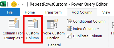
1. In the Power Query Editor, click the “Add Column” tab
2. Click on “Custom Column” option

3. In the “New column name” field, enter any name you prefer. I will leave it as Custom
4. In the formula field, type: {1..[Rept]} (where “[Rept]” is the name of your column that contains the repeat count) Tip: You can either type this manually or simply double-click on the column name in the “Available columns” list to insert it.

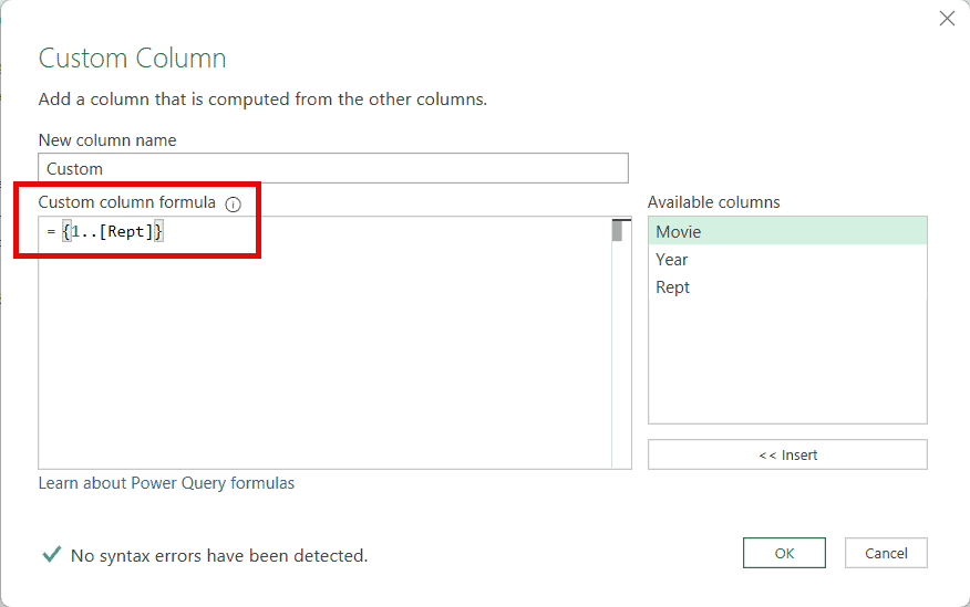
5. Click OK

Once done, you will see that the new column displays a “List” value in each cell (as shown below).

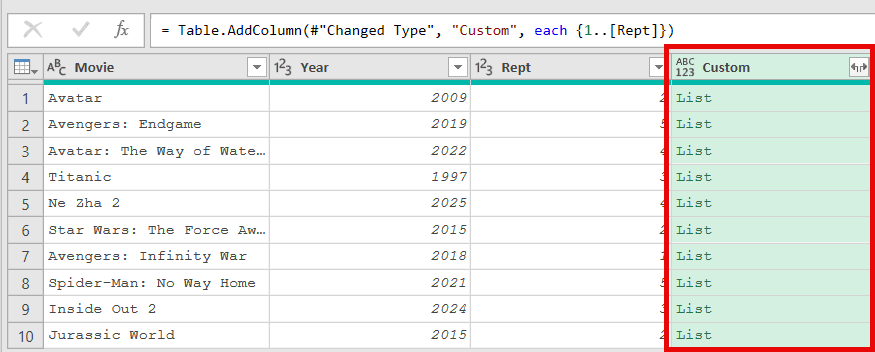
If you click on the first row’s list, you will see it contains [1, 2] because the Rept column value for that row was 2.

The second row will show [1, 2, 3, 4, 5] because its Rept column value for that row was 5, and so on.

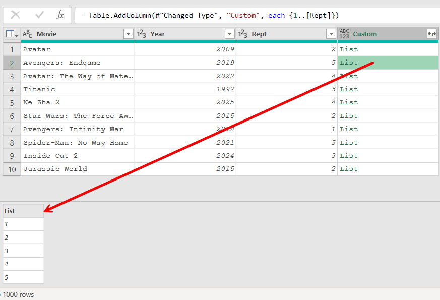
What’s happening is that Power Query is creating a custom-sized list for each row based on the values in your Rept column. Pretty neat, right?

Step 4: Expand the List to Rows

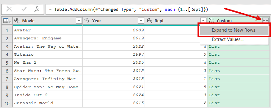
Now let’s expand these dynamic lists:

1. Click the expand icon (two diagonal arrows) on your new custom column
2. Select “Expand to New Rows”

And just like that, the magic happens! Each row has been repeated exactly the number of times specified in the Rept column.

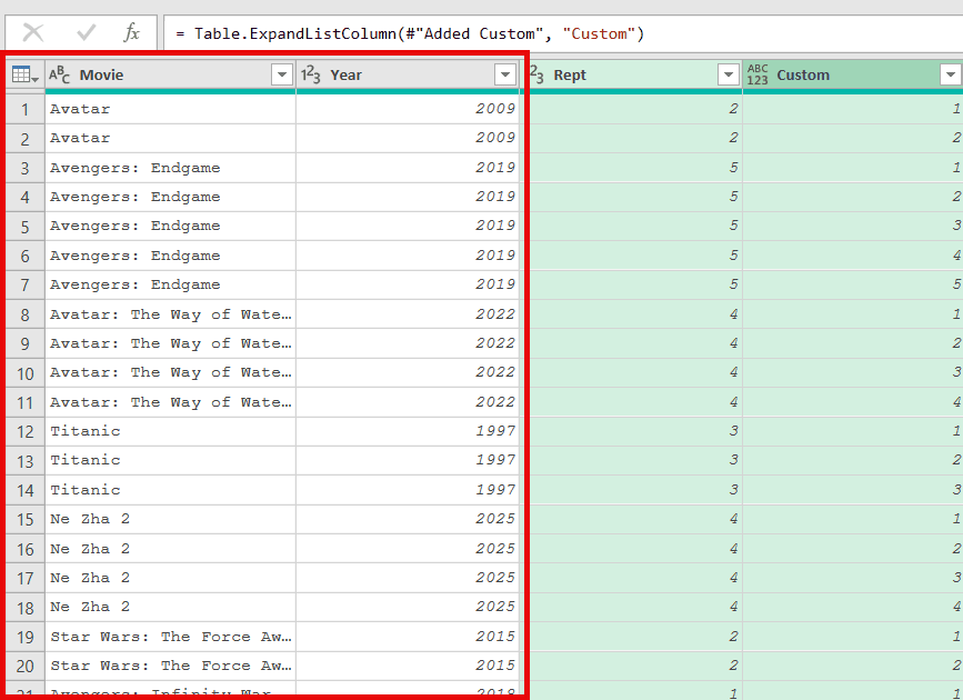
Pretty Neat… isn’t it!

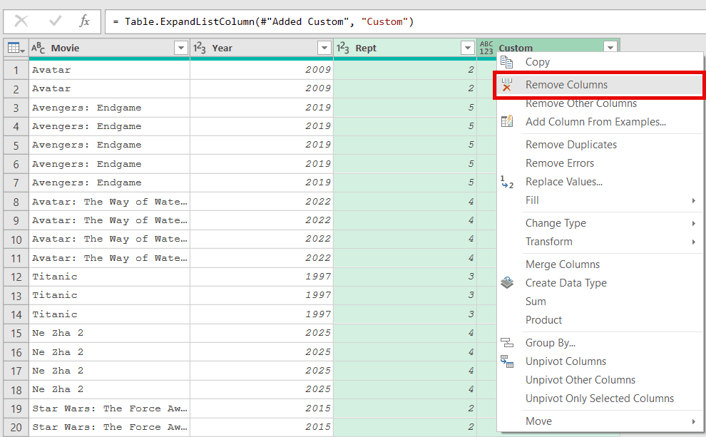
Step 5: Remove Unnecessary Columns

Now let’s clean up our data:

1. Right-click on the custom column header and select “Remove”
2. If you also want to remove the original Rept column (the one that specified the repeat count), right-click on it and select “Remove”

Now we have the result that we wanted. The only step left now is to get this data in Excel.

Step 6: Load the Data to Excel

Follow the below steps to get the data in Excel as a Table:

1. Go to File tab
2. Click on Close & Load

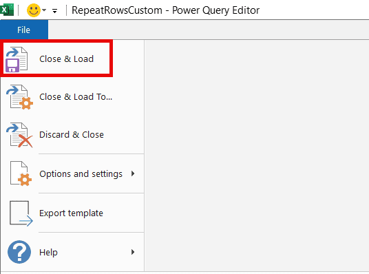
This will insert a new sheet into your Excel workbook and the resulting data will be inserted as an Excel Table.

And just like the previous method, if you make any changes in the original table, you can get the updated result by simply refreshing the query result. To do that, right-click on any cell in the result table and the click on Refresh

So this is how you can use Power Query to repeat rows in Excel N times or based on a value in a column.

I hope you found this article helpful.

Other Excel articles you may also like:

• How to Print the Top Row on Every Page in Excel (Repeat Row/Column Headers)
• Prevent Duplicate Entries in Excel
• Convert Columns to Rows in Excel
• How to Move Rows and Columns in Excel