
The Table.Group function groups rows in a table based on one or more columns and applies aggregations to each group.
Think of it as the Power Query equivalent of a pivot table.
You tell it which column(s) to group by, and what calculations to perform on each group (sum, count, average, etc.).
It’s one of the most commonly used functions in Power Query, and once you understand how it works, you can handle most data summarization tasks with ease.
Table.Group Syntax
= Table.Group(table as table, key as any, aggregatedColumns as list, optional groupKind as nullable number, optional comparer as nullable function) as table
- table – The source table you want to group
- key – The column name (as text) or a list of column names to group by. For example, “Region” or {“Region”, “Product”}
- aggregatedColumns – A list defining the new columns to create from each group. Each item is a list with 2 or 3 elements: {NewColumnName, AggregationFunction} or {NewColumnName, AggregationFunction, DataType}
- groupKind (optional) – Controls how rows are grouped. GroupKind.Global (default) groups all matching rows across the entire table. GroupKind.Local groups only consecutive matching rows
- comparer (optional) – A custom comparison function that determines how key values are matched. For example, Comparer.OrdinalIgnoreCase for case-insensitive grouping
What it returns: A new table with one row per group, containing the key column(s) and the aggregated columns you defined.
When to Use Table.Group
Use this function when you need to:
- Summarize data by category (total sales by region, average price by product)
- Count rows per group (number of orders per customer)
- Perform multiple aggregations in a single step (sum, average, min, max together)
- Concatenate text values within each group (combine names into a comma-separated list)
- Get all rows belonging to each group as a nested table for further transformation
- Find the top or bottom value within each group
- Detect consecutive periods or streaks in your data (using GroupKind.Local)
Example 1: Basic Grouping with Sum
Let’s start with the most common use case. You have sales data and want to find the total sales for each region.
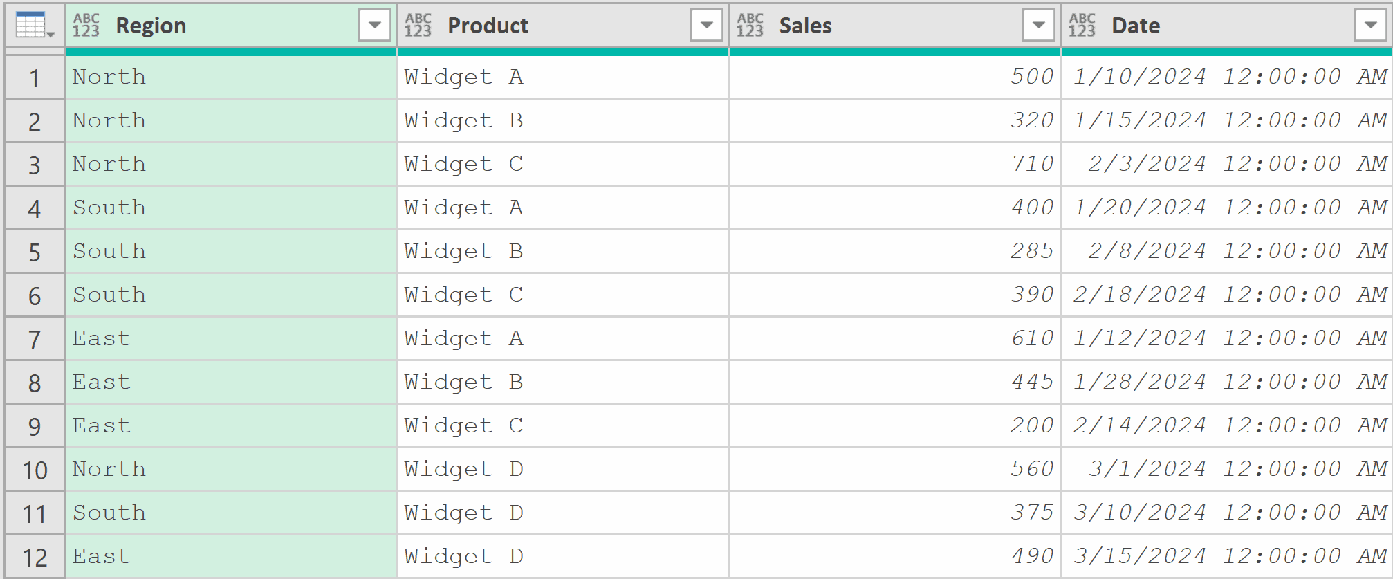
Suppose you have a table with columns Region, Product, and Sales, and you want to group by Region to get the total sales per region.
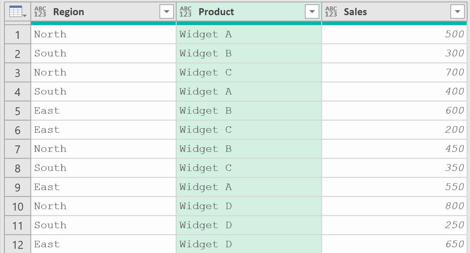
Add a new step (by clicking on the fx icon next to the formula bar) and use this formula:
= Table.Group(Source, {"Region"}, {{"Total Sales", each List.Sum([Sales]), type number}})
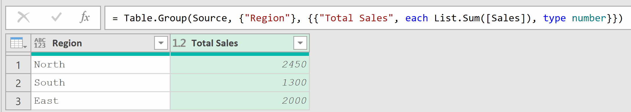
In the above example, the function groups all rows by the Region column. For each group, List.Sum([Sales]) adds up all the Sales values.
The each keyword is important here. Inside the aggregation, each refers to the sub-table of rows belonging to that group.
So [Sales] gives you a list of all Sales values within that group, and List.Sum adds them up.
The third element type number tells Power Query that the resulting column contains numbers.
You can also do the same thing using the user interface by using the steps below:
- In the Home tab, click on the Group By icon.
- In the Group By dialog box, make the following changes:
- Select Region as the column to group by.
- Use Total Sales as the name for the new column
- Select Sum as the operation.
- Select the Sales column to apply the operation to.
- Click OK
Example 2: Counting Rows Per Group
Here’s another common use case. You want to count how many orders each customer has placed.
Suppose you have an Orders table with columns Customer Name, Order Date, and Amount.
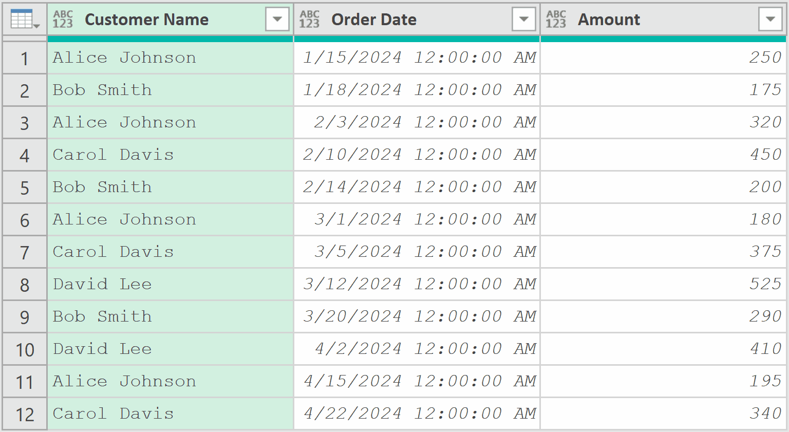
Add a new step (by clicking on the fx icon next to the formula bar) and use this formula:
= Table.Group(Source, {"Customer Name"}, {{"Order Count", each Table.RowCount(_), Int64.Type}})
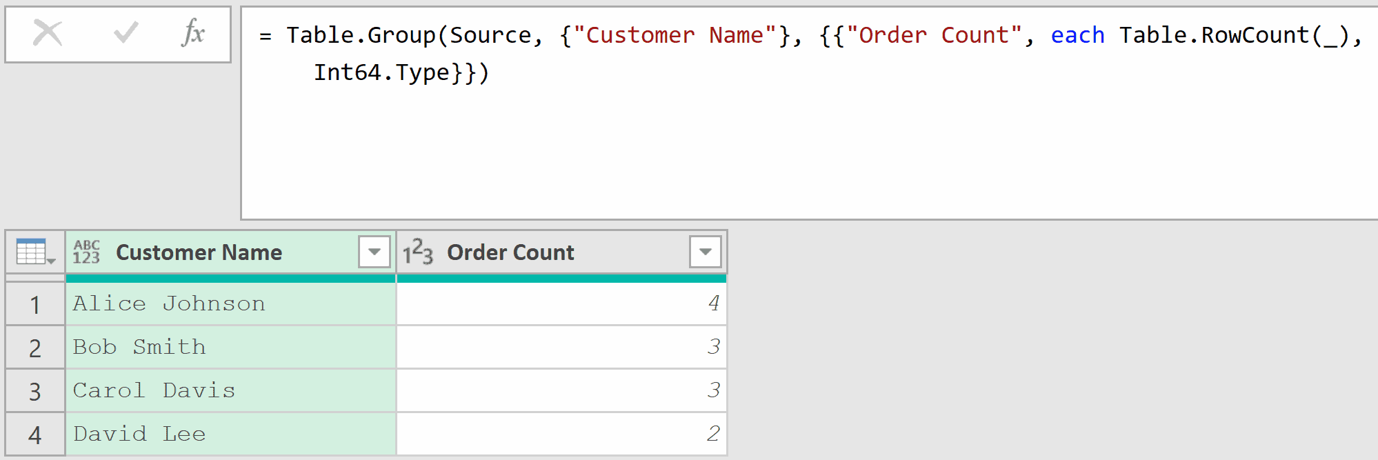
Here, Table.RowCount(_) counts the number of rows in each group’s sub-table. The underscore _ represents the entire sub-table for that group (it’s what each passes implicitly).
You could also use List.Count([Order Date]) instead of Table.RowCount(_) and it would give you the same result.
You can also do the same thing using the user interface by using the steps below:
- In the Home tab, click on the Group By icon.
- In the Group By dialog box, make the following changes:
- Select Customer Name as the column to group by.
- Use Order Count as the name for the new column
- Select Count Rows as the operation.
- Click OK
Example 3: Multiple Aggregations at Once
Now let’s tackle something more powerful.
Instead of calculating just one thing per group, you can calculate multiple aggregations in a single step.
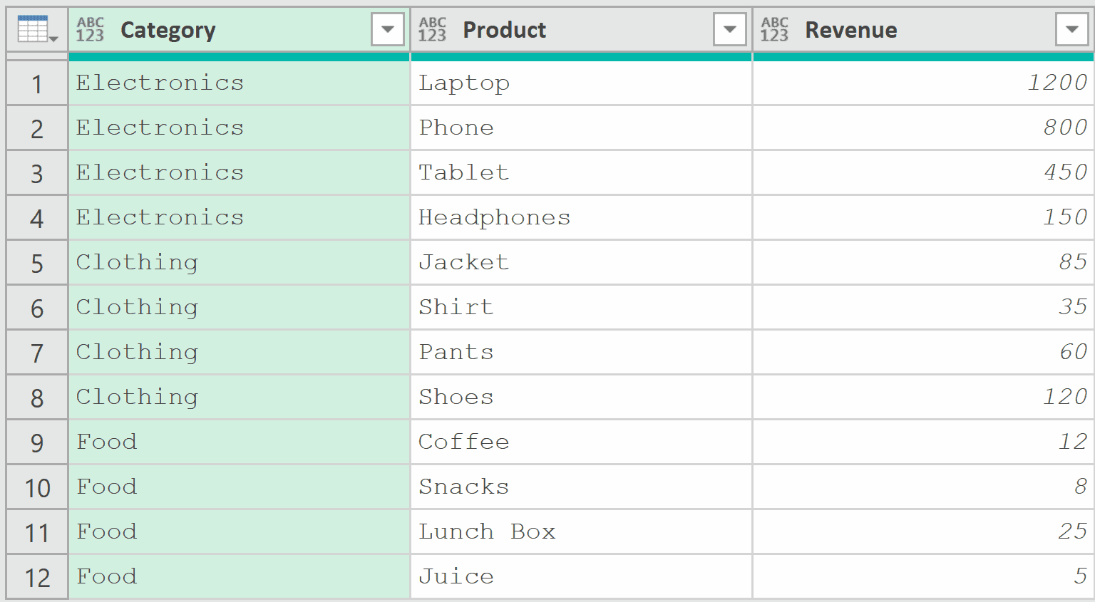
Suppose you have a Sales table with columns Category, Product, and Revenue, and you want to get the total, average, minimum, maximum revenue, and count for each category.
Add a new step (by clicking on the fx icon next to the formula bar) and use this formula:
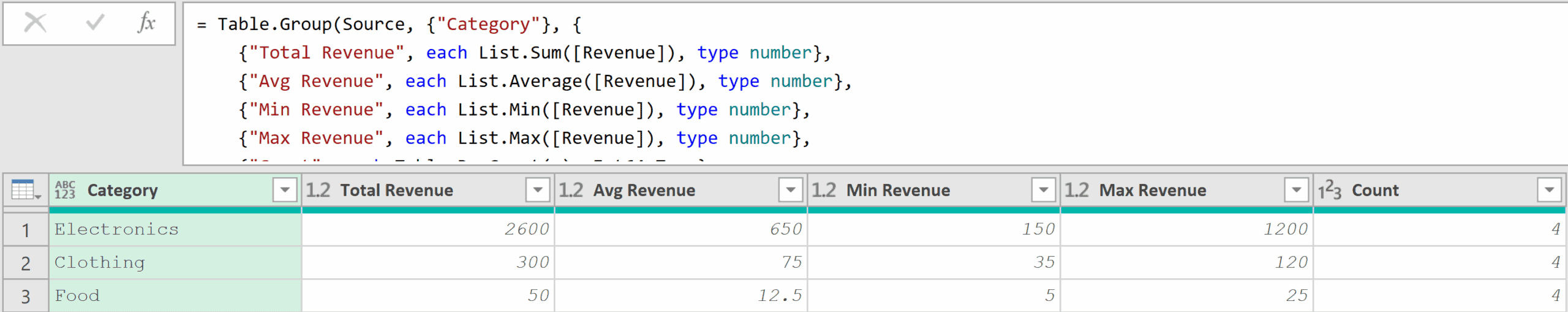
= Table.Group(Source, {"Category"}, {
    {"Total Revenue", each List.Sum([Revenue]), type number},
    {"Avg Revenue", each List.Average([Revenue]), type number},
    {"Min Revenue", each List.Min([Revenue]), type number},
    {"Max Revenue", each List.Max([Revenue]), type number},
    {"Count", each Table.RowCount(_), Int64.Type}
})
Result: A table with one row per category, showing all five aggregated columns.
Each aggregation is defined as a separate list inside the outer list.
You can add as many aggregations as you need. Just follow the pattern: {“Column Name”, each AggregationFunction([Column]), DataType}.
You can also do the same thing using the user interface by using the steps below:
- In the Home tab, click on the Group By icon.
- In the Group By dialog box, make the following changes:
- Select the Advanced Option
- Select Category as the column to group by.
- Add New column name, operation and column as shown below
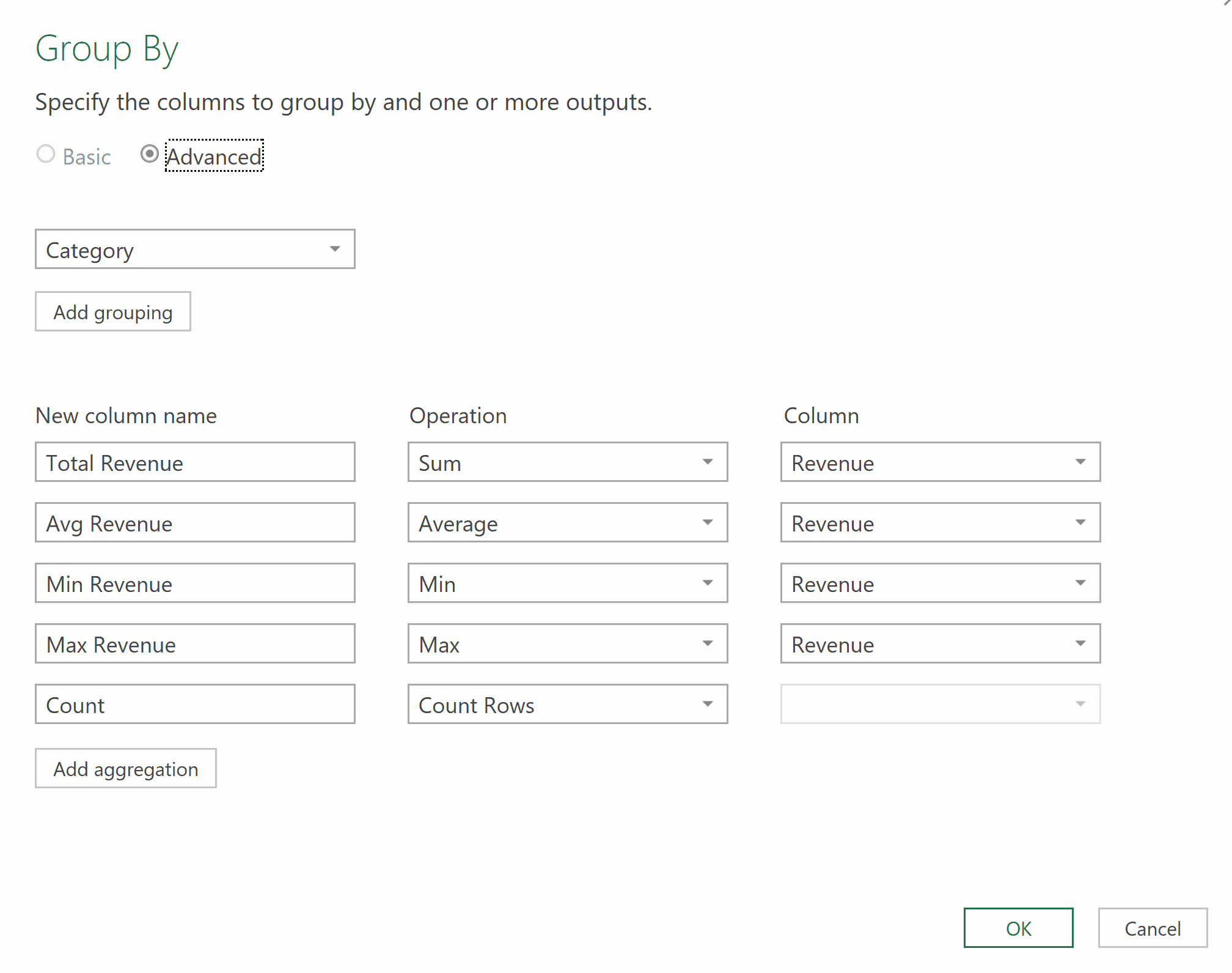
- Click OK
Example 4: Grouping by Multiple Columns
This next one comes up quite often. Sometimes grouping by a single column isn’t enough, and you need to group by two or more columns.
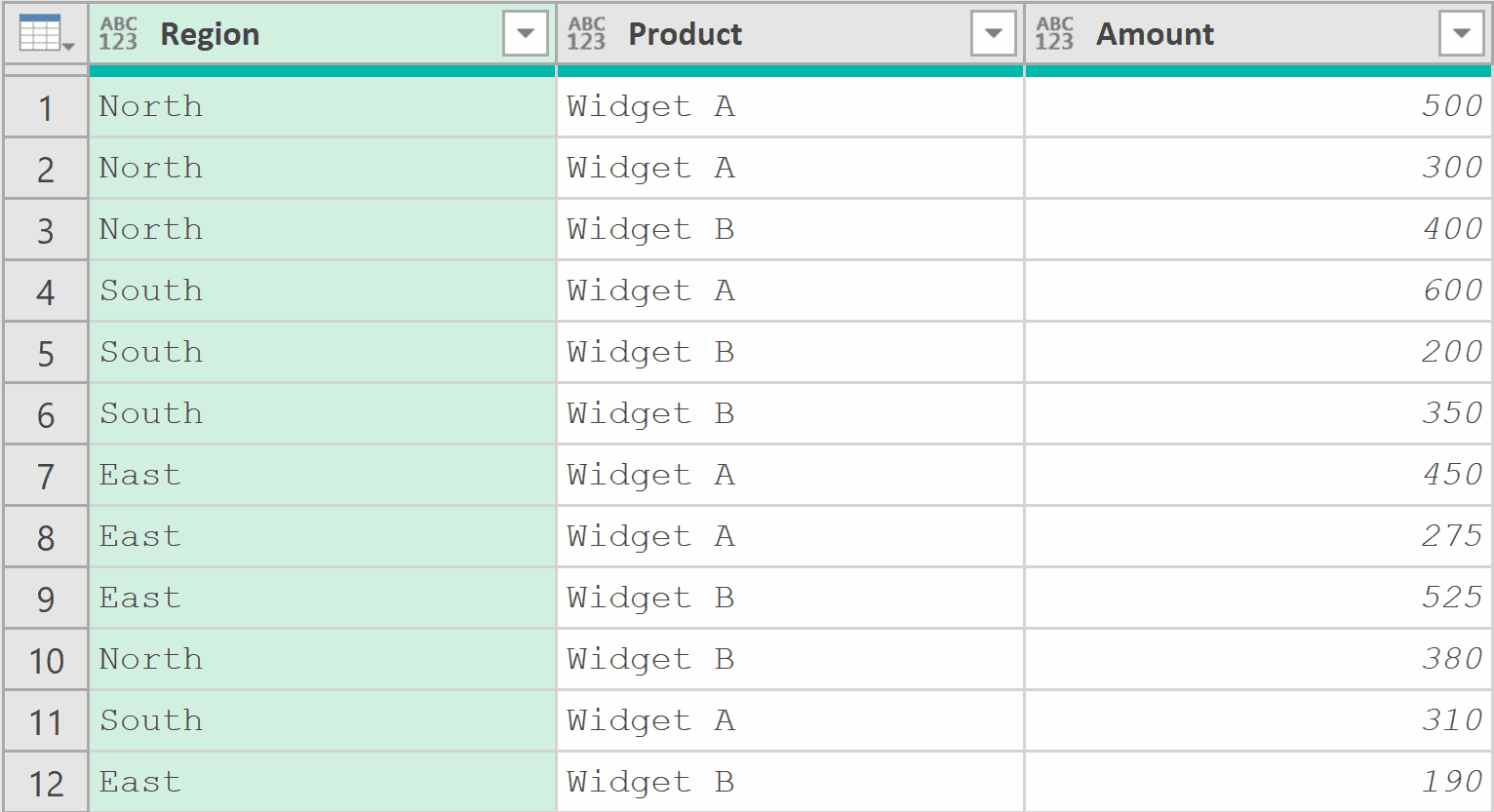
Suppose you have a Sales table with columns Region, Product, and Amount, and you want to get the total amount for each Region-Product combination.
Add a new step (by clicking on the fx icon next to the formula bar) and use this formula:
= Table.Group(Source, {"Region", "Product"}, {{"Total Amount", each List.Sum([Amount]), type number}})
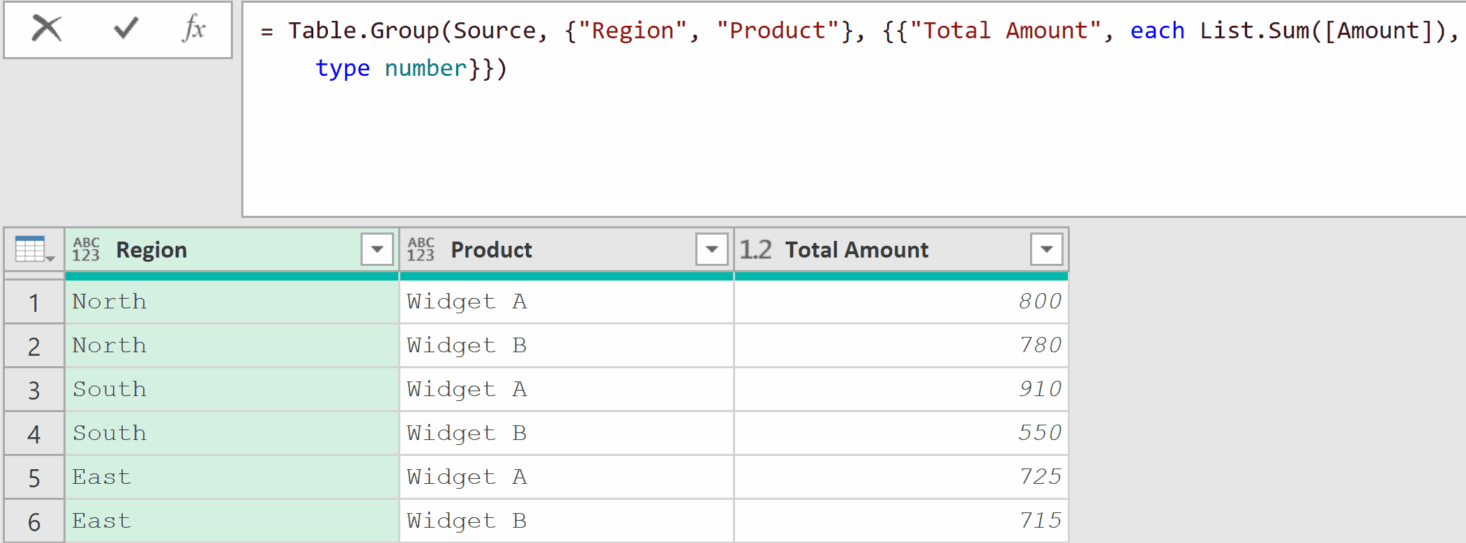
The key difference from the previous examples is that the second argument is now a list of multiple column names {“Region”, “Product”} instead of a single column name.
This tells the function to create a unique group for each combination of Region and Product.
You can also do the same thing using the user interface by using the steps below:
- In the Home tab, click on the Group By icon.
- In the Group By dialog box, make the following changes:
- Select the Advanced option
- Select Region as the column to group by.
- Then select Product as the next column to group by
- Use Total Amount as the name for the new column
- Select Sum as the operation.
- Select the Amount column to apply the operation to.
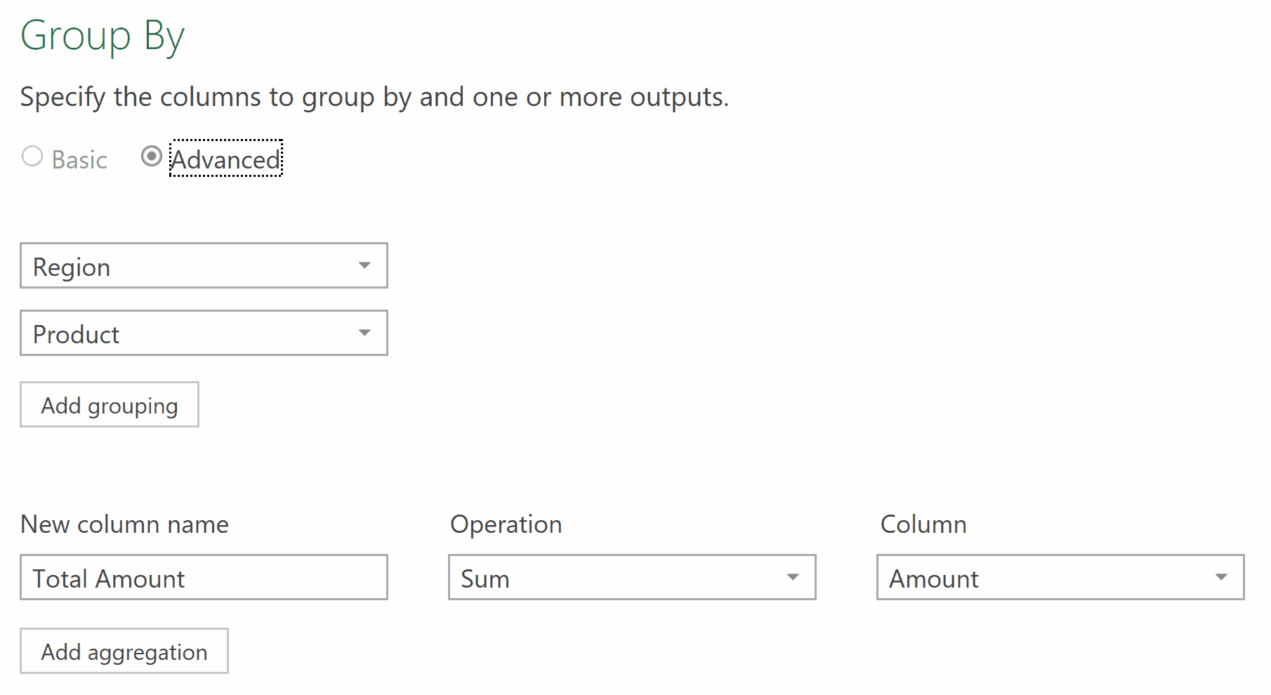
- Click OK
Example 5: Concatenating Text Values Per Group
Here’s a really useful one. Suppose you want to combine multiple text values from each group into a single comma-separated string.
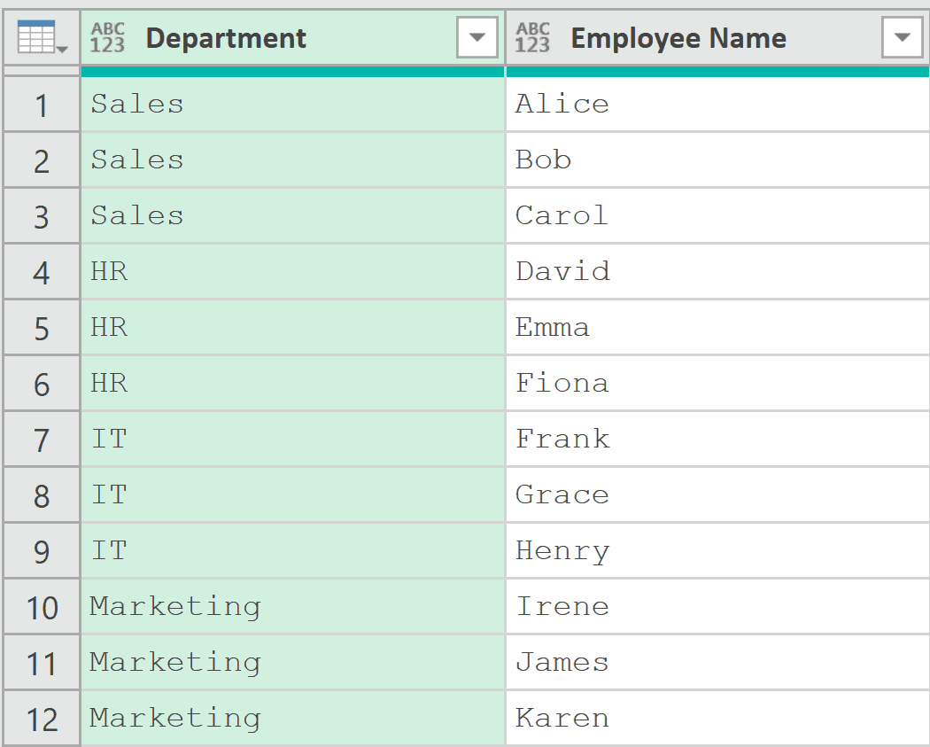
For example, you have a table with Department and Employee Name, and you want a single row per department showing all employee names.
Add a new step (by clicking on the fx icon next to the formula bar) and use this formula:
= Table.Group(Source, "Department", {{"Employees", each Text.Combine([Employee Name], ", "), type text}})
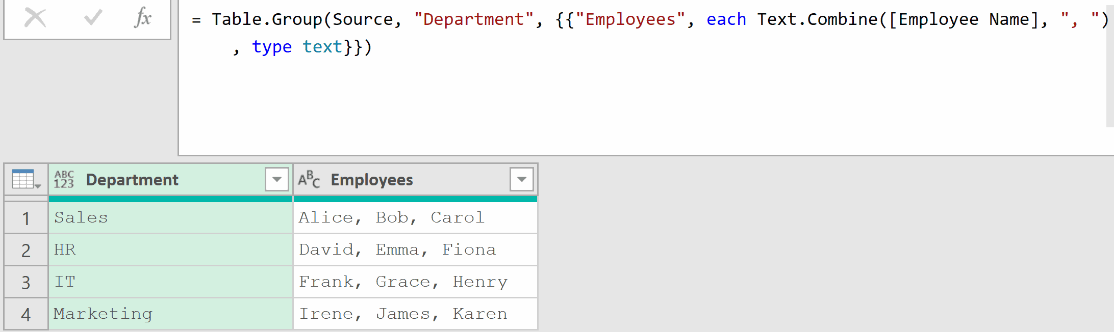
In this example, [Employee Name] gives a list of all employee names in each group. Text.Combine then joins them together with “, ” as the separator.
This is really handy when you need to flatten a one-to-many relationship into a single cell.
Note: This is something that you cannot do with the user interface, as we are first grouping by department names and then concatenating all the names in the new Employees column
Example 6: Getting All Rows as a Nested Table
This is a foundational technique for advanced Power Query work. Instead of aggregating values, you can keep the entire sub-table for each group.
Suppose you have a Sales table and you want to group by Region, but keep all the original rows accessible within each group.
Add a new step (by clicking on the fx icon next to the formula bar) and use this formula:
= Table.Group(Source, {"Region"}, {{"AllData", each _, type table}})
Result: A table with one row per region, and a column called AllData that contains nested tables.
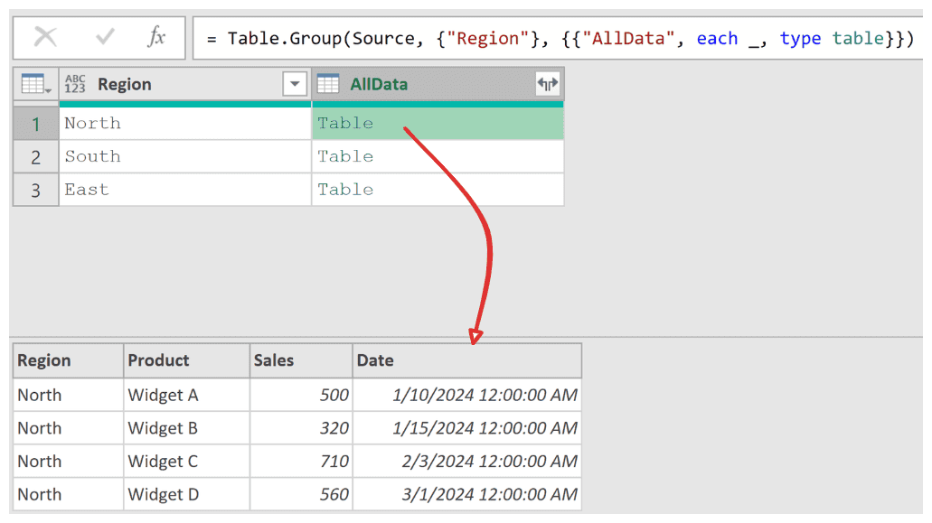
The magic here is each _. The underscore represents the full sub-table for that group. So instead of calculating a sum or count, you’re storing the entire set of rows.
You can click on the white space next to any nested table value to preview its contents at the bottom of the Power Query Editor.
This technique is powerful because you can then apply transformations to each nested table individually (like sorting, filtering, or adding index columns) before combining them back together.
You can also do the same thing using the user interface by using the steps below:
- In the Home tab, click on the Group By icon.
- In the Group By dialog box, make the following changes:
- Select Region as the column to group by.
- Use AllData as the name for the new column
- Select All Rows as the operation.
- Click OK
Example 7: Finding Top Value Per Group
Now let’s build on the nested table concept.
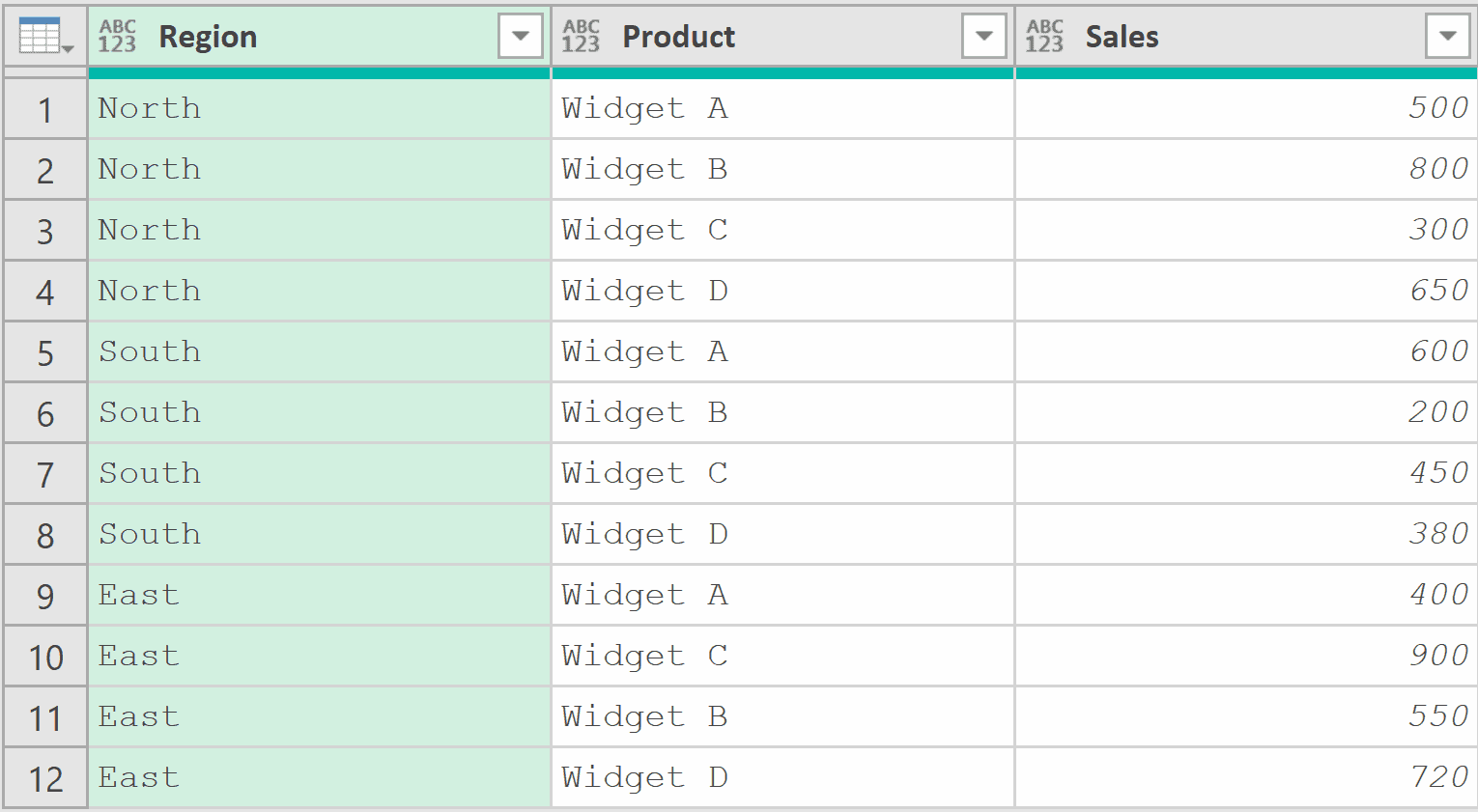
Suppose you want to find the highest-selling product in each region.
You have a Sales table with columns Region, Product, and Sales (as shown below).
With the table loaded in Power Query, add a new step (by clicking on the fx icon next to the formula bar) and use this formula:
= Table.Group(Source, "Region", {
    {"Top Product", each Table.Max(_, "Sales")[Product], type text},
    {"Max Sales", each List.Max([Sales]), type number}
})
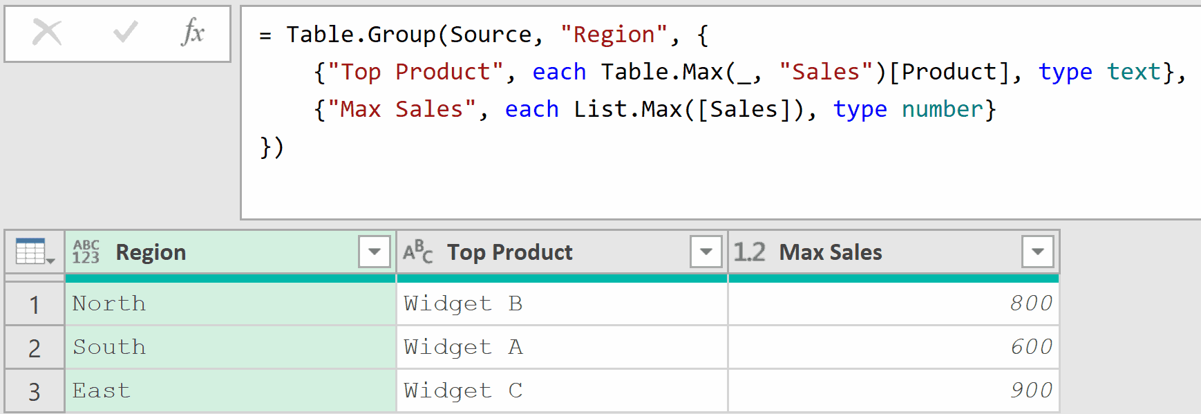
Here, Table.Max(_, “Sales”) returns the entire row with the highest Sales value within each group. Adding [Product] at the end extracts just the Product name from that row.
The second aggregation is List.Max([Sales]) that gives the maximum sales for each region.
Example 8: GroupKind.Local for Consecutive Groups
This is where Table.Group gets really interesting.
The fourth parameter, GroupKind.Local, changes how grouping works. Instead of grouping all matching rows across the entire table, it only groups consecutive rows that share the same key value.
Suppose you have an employee activity log that tracks daily status.
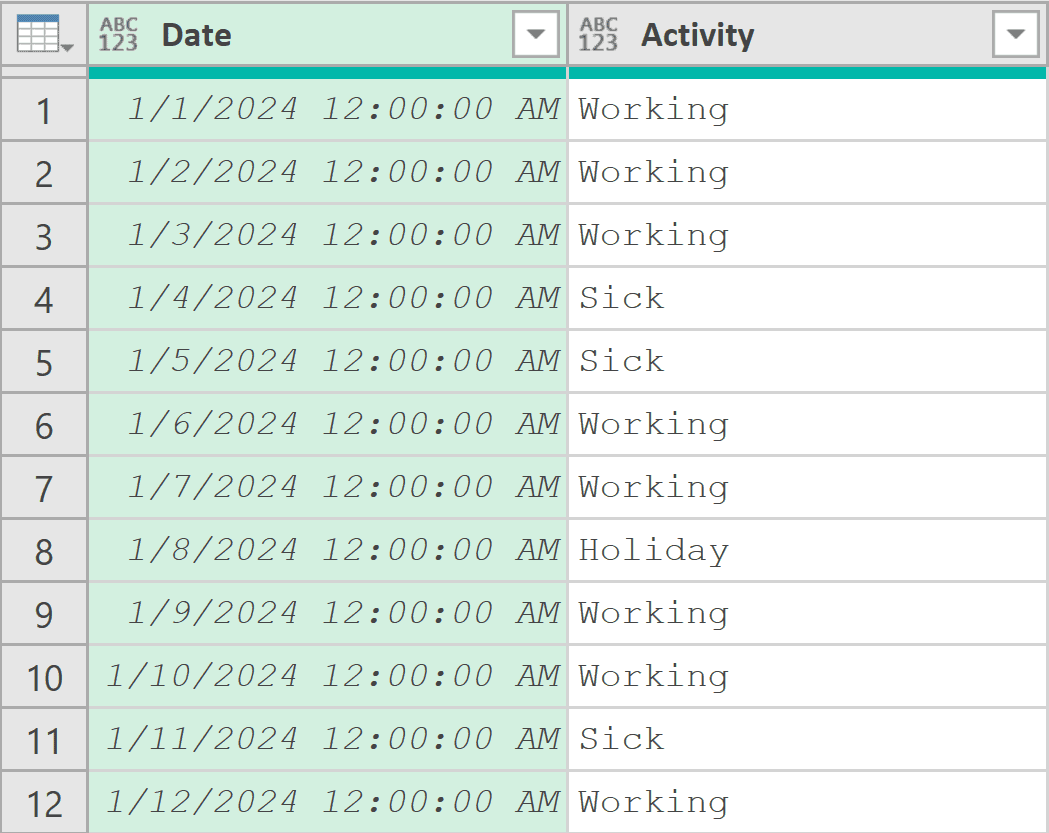
Notice that “Working” appears in three separate stretches (Jan 1-3, Jan 6-7, and Jan 9).
With the default GroupKind.Global, all “Working” rows would be lumped into one group.
But with GroupKind.Local, each contiguous stretch becomes its own group.
Add a new step (by clicking on the fx icon next to the formula bar) and use this formula:
= Table.Group(Source, "Activity", {
    {"Start Date", each Date.From(List.Min([Date])), type date},
    {"End Date", each Date.From(List.Max([Date])), type date},
    {"Days", each Table.RowCount(_), Int64.Type}
}, GroupKind.Local)
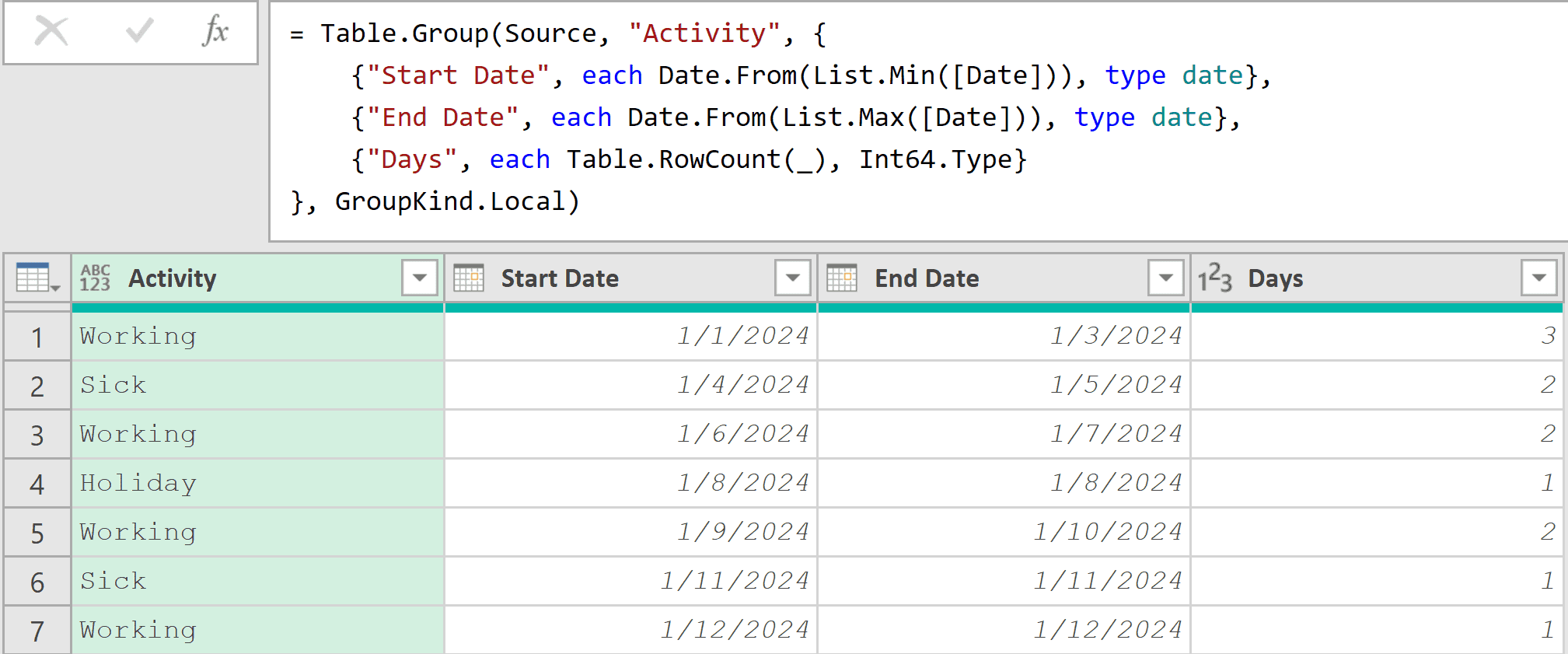
The result shows five separate groups instead of three. Each contiguous stretch of the same activity gets its own row with start date, end date, and duration.
This is incredibly useful for detecting streaks, shifts, or any scenario where the sequence of data matters.
Pro Tip: The type date declaration in the aggregation list only sets the column’s metadata. This means that it tells Power Query what type the column should contain, but it doesn’t actually convert the values in the column itself. If your source column contains datetime values, List.Min and List.Max will return datetime values regardless of the type annotation. To actually strip the time component, you need to explicitly convert the values using Date.From().
Important: GroupKind.Local only works correctly when your data is already sorted by the key column(s). If the data isn’t sorted, sort it first using Table.Sort before applying the group.
Performance Note: When your data is already sorted by the key columns, using GroupKind.Local can also give you a performance boost. Since Power Query knows that all rows with the same key value will appear together, it doesn’t need to scan through the entire table to find matching rows. This can make a noticeable difference when working with large datasets.
Example 9: Case-Insensitive Grouping with Custom Comparer
And finally, let’s look at the fifth parameter of the Table.Group function.
By default, Table.Group uses case-sensitive comparison when matching key values. This means “Electronics” and “electronics” would be treated as separate groups.
Suppose you have product data where category names are inconsistently capitalized.

With the table loaded in Power Query, add a new step (by clicking on the fx icon next to the formula bar) and use this formula:
= Table.Group(Source, {"Category"}, {
    {"TotalPrice", each List.Sum([Price]), type number},
    {"Count", each Table.RowCount(_), Int64.Type}
}, GroupKind.Global, Comparer.OrdinalIgnoreCase)
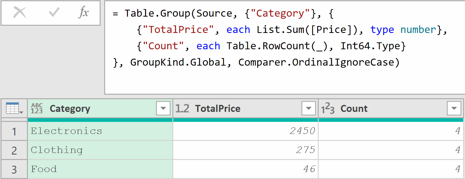
Without the comparer, you would get three separate groups for Electronics, electronics, and ELECTRONICS.
The Comparer.OrdinalIgnoreCase parameter tells the function to ignore case differences when matching key values.
Note that the Category value in the result comes from the first row encountered in each group. So the capitalization of the output depends on whichever row appears first.
Tips & Common Mistakes
- Understand each and _: Inside the aggregation function, _ (the implicit parameter of each) represents the sub-table for that group, not a single row. So [Sales] gives you a list of all Sales values in the group, and _ gives you the entire sub-table. This is the most common source of confusion.
- Always specify data types: Use the three-element format {“ColumnName”, each …, type number} instead of just {“ColumnName”, each …}. Omitting the type can cause issues downstream, especially in Power BI data models.
- Row order is not guaranteed: Table.Group does not guarantee the order of rows in the result. If you need sorted output, add a Table.Sort step after the grouping step.
- Sort before using GroupKind.Local: GroupKind.Local only groups consecutive rows. If your data isn’t sorted by the key column, you’ll get fragmented groups. Always add a Table.Sort step before using Local grouping.
- Group By UI generates Table.Group code: The Group By button in the Power Query ribbon is just a visual interface for this function. Click it to build basic groupings through the UI, then modify the generated M code in the formula bar for advanced scenarios.
- Use each _ for complex transformations: When you need to do something beyond simple aggregation (like ranking within groups or applying conditional logic), group with each _ first to get nested tables, transform each one, then combine them back with Table.Combine.
Other Related Power Query Functions
- Table.RenameColumns – Change one or more column names in a table
- Table.TransformColumns – Apply transformations to one or more columns in a table simultaneously
- Table.Buffer – Loads a table into memory so Power Query reads from the cached copy.
- Table.Sort – Sorts a table by one or more columns
- Table.Combine – Combines multiple tables into one
- List.Count – Returns the total number of items in a list.
All Power Query Functions


