List.Transform Function in Power Query M

If you want to run the same change on every item in a list in Power Query, the List.Transform function is what you’re looking for. It takes a list and a function, applies that function to each item, and gives you back a new list of the results.

In this article, I’ll walk you through List.Transform with practical examples: tweaking numbers, cleaning up text, converting values to a new format, and even numbering a list using its own positions.

List.Transform Function Syntax

List.Transform(list as list, transform as function) as list

• list – The list whose items you want to change
• transform – The function applied to each item, one at a time

What it returns: A new list, the same length as the input, where each item is the result of running the transform function on the matching input item. The order is preserved.

When to Use List.Transform

Use this function when you need to:

• Apply the same calculation to every number in a list
• Clean or reformat every value in a text column
• Convert a list of values into a new shape (add a prefix, pad with zeros, tag with a label)
• Turn one column of a table into a transformed list
• Build a numbered or indexed list using each item’s position

Example 1: Transform Every Item in a List

Let’s start with a basic example. The simplest way to see List.Transform in action is to feed it a list of numbers and add the same amount to each one.

Create a new blank query (Data > Get Data > From Other Sources > Blank Query), open Home > Advanced Editor, and replace everything in it with this code:

let
    Source = List.Transform({10,20,30,40},each _ + 5)
in
    Source

Result: a list containing 15, 25, 35, 45

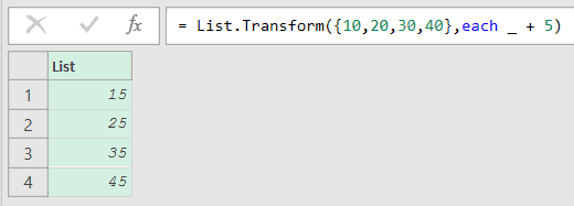
Here, {10,20,30,40} is the starting list, and each _ + 5 is the transform. The each keyword turns _ + 5 into a small function, and _ stands for the current item, so List.Transform walks the list and adds 5 to every number.

The preview shows a List of the four results in the same order as the input.

Example 2: Apply a Discount to a Price Column

Here’s a common use. You have a column of prices in a table and you want to knock a percentage off each one.

Suppose you have a Products table with a Product and a Price column, and you want a list of prices after a 10% discount.

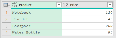
Load this table into Power Query (select any cell in it, then go to Data > From Table/Range), and it adds a “Changed Type” step that sets Price to a number. Add a new step after it (click the fx icon next to the formula bar) and use this formula:

= List.Transform(#"Changed Type"[Price], each _ * 0.9)

Result: a list containing 108, 40.5, 234, 76.5

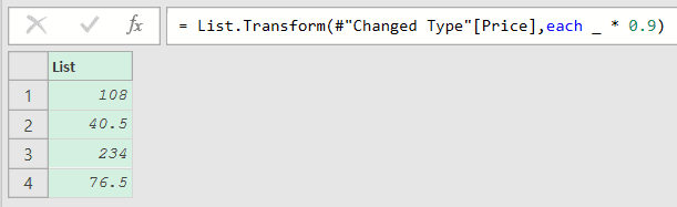
In this formula, #"Changed Type"[Price] grabs the Price column as a list (the #"..." wrapper is how M writes a step name with a space in it). List.Transform then multiplies each price by 0.9, which is the same as taking 10% off.

Example 3: Capitalize Every Value in a Text Column

This next one comes up a lot in data cleaning. You have a column of text in lowercase and you want each value properly capitalized.

Suppose you have a Cities table with a single City column where the names are all lowercase, and you want them in title case.

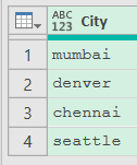
Load this table into Power Query the same way as in Example 2. This time the formula reads the City column straight from Source, the query’s first step.

If your query has a “Changed Type” step, #"Changed Type"[City] works too and gives the same result, since that step leaves text values unchanged.

Add a new step (by clicking on the fx icon next to the formula bar) and use this formula:

= List.Transform(Source[City], Text.Proper)

Result: a list containing Mumbai, Denver, Chennai, Seattle

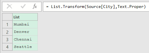
Notice there’s no each here. Instead of writing each Text.Proper(_), I passed the Text.Proper function by name and List.Transform hands each item to it automatically.

That shortcut works whenever your transform is a single function that takes one argument. It’s cleaner than the each version and does the exact same thing.

Example 4: Pull the First Name from a Full Name

Here’s another handy one for text. You have a list of full names and you want just the first name from each.

Suppose you have an Employees table with a Full Name column, and you want a list of only the first names.

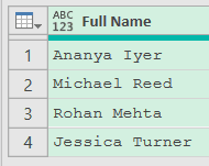
Like Example 3, the formula reads the Full Name column straight from Source. If your query has a “Changed Type” step, #"Changed Type"[Full Name] works too.

Add a new step (by clicking on the fx icon next to the formula bar) and use this formula:

= List.Transform(Source[Full Name], each Text.BeforeDelimiter(_, " "))

Result: a list containing Ananya, Michael, Rohan, Jessica

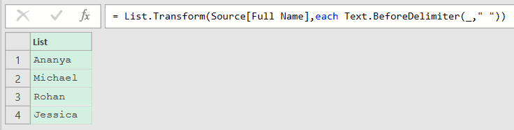
Here, Text.BeforeDelimiter(_," ") grabs everything before the first space in each name. List.Transform runs it on every value, so you end up with a clean list of first names.

This time the transform needs an extra argument (the space), so each is required. You can’t use the bare-function shortcut from Example 3 when you have to pass more than the item itself.

Example 5: Add a Prefix to Order Numbers

Let’s convert values into a new format. You have a column of plain order numbers and you want each one turned into a proper order code with a prefix.

Suppose you have an Orders table with an Order No column of numbers, and you want a list like ORD-4501 for each.

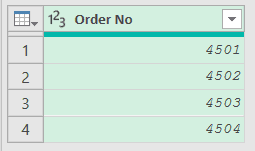
Loading this table adds a “Changed Type” step that sets Order No to a number. Add a new step after it (click the fx icon next to the formula bar) and use this formula:

= List.Transform(#"Changed Type"[Order No], each "ORD-" & Text.From(_))

Result: a list containing ORD-4501, ORD-4502, ORD-4503, ORD-4504

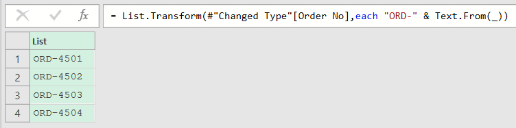
Here, Text.From(_) turns each number into text so it can be joined, and "ORD-" & ... sticks the prefix on the front. List.Transform builds the full code for every row.

If you want to stitch a whole list into one string instead of transforming each item, the Text.Combine function is the one to reach for.

Example 6: Convert Scores into Pass or Fail Labels

List.Transform is great for turning values into labels with a bit of logic. Let’s mark each score as a pass or a fail.

Suppose you have a Scores table with a Student and a Score column, and you want a list that says Pass for 50 and above, or Fail below that.

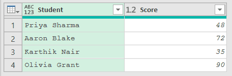
Loading this table adds a “Changed Type” step that sets Score to a number. Add a new step after it (click the fx icon next to the formula bar) and use this formula:

= List.Transform(#"Changed Type"[Score], each if _ >= 50 then "Pass" else "Fail")

Result: a list containing Fail, Pass, Fail, Pass

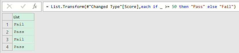
Here, the transform is an if statement. For each score, it checks whether the value is 50 or more and returns “Pass” or “Fail” accordingly.

You can put any expression you like inside each, including full if ... then ... else logic, as long as it returns a value.

Example 7: Build a Numbered List Using Positions

Now let’s tackle something a bit more advanced. You want to number a list, like a ranking, where each item is prefixed with its position.

Suppose you have a Finishers table with a Runner column, and you want a numbered list: “1. Neha Kapoor”, “2. Daniel Brooks”, and so on.

Like Example 3, the formula reads the Runner column straight from Source. If your query has a “Changed Type” step, you can also replace both Source references in the formula below with #"Changed Type".

Add a new step (by clicking on the fx icon next to the formula bar) and use this formula:

= List.Transform(List.Positions(Source[Runner]), each Text.From(_ + 1) & ". " & Source[Runner]{_})

Result: a list containing 1. Neha Kapoor, 2. Daniel Brooks, 3. Vikram Rao

List.Transform only hands the transform each item’s value, never its position, so this formula transforms the positions instead. List.Positions(Source[Runner]) gives you the position list 0, 1, 2, one number for each runner.

Inside the transform, _ is the position, so Text.From(_ + 1) builds the human number (starting at 1, not 0) and Source[Runner]{_} pulls the runner at that position. Joining the two with “. ” in between gives the numbered line.

Example 8: Pad Codes with Leading Zeros

One more reformatting example. You have short numeric codes and you want them all the same width, padded with leading zeros.

Suppose you have a Codes table with a Region Code column, and you want every code shown as three digits, like 012 or 007.

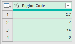
Loading this table adds a “Changed Type” step that sets Region Code to a number. Add a new step after it (click the fx icon next to the formula bar) and use this formula:

= List.Transform(#"Changed Type"[Region Code], each Text.PadStart(Text.From(_), 3, "0"))

Result: a list containing 012, 007, 034, 009

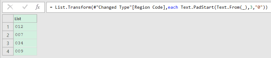
Here, Text.From(_) turns each code into text, and Text.PadStart(...,3,"0") pads it on the left with zeros until it’s three characters wide. So 12 becomes 012 and 7 becomes 007.

Tips & Common Mistakes

• each _ vs passing a function by name: When your transform is a single one-argument function, you can pass it by name (Text.Proper) instead of wrapping it in each Text.Proper(_). Both work, but switch back to each the moment you need a second argument or extra logic.
• There’s no built-in index argument: List.Transform doesn’t hand your transform a position number. If you need the index (for ranking, numbering, or reaching back into another list), transform List.Positions(yourList) instead and index into the original list inside the function, as shown in Example 7.
• Nulls are passed through, not skipped: List.Transform runs the transform on every item, including nulls. Text.Proper just returns null for a null, so a text cleanup like Example 3 keeps going.
• Comparisons break on nulls: The Pass/Fail check from Example 6 errors on a null (“We cannot convert the value null to type Logical”), because null >= 50 gives null instead of true or false. Guard it with each if _ = null then null else if _ >= 50 then "Pass" else "Fail", which leaves the null in place and labels everything else.
• The output list is the same length as the input: List.Transform never adds or drops items, so the result always has one entry per input item. You can confirm this with the List.Count function if you’re ever unsure.
• It always returns a list, not a table: The output is a list of values, even when the input came from a table column. If you need the results as a table, select List Tools > Transform > To Table.
• Need a new column instead? Skip List.Transform and use Add Column > Custom Column on the original table. For the Example 2 discount, the custom column formula is [Price] * 0.9, with the column name [Price] taking the place of _.

Related Power Query Functions / Articles:

• List.Contains – Checks whether a specific value exists in a list
• List.IsDistinct – Checks if every value in a list is unique, returning true or false
• List.Dates – Generates a list of dates from a start date, count, and step size
• Table.TransformColumns – Applies a transform function to one or more columns of a table
• List.Generate function
• Table.ReplaceValue
• Text.PadStart Function in Power Query M
• List.Select – Use List.Select in Power Query M to keep only the list items that meet a condition.

All Power Query Functions