
A growing annuity is a series of payments where the amount goes up by the same percentage every period.
Something like a pension that rises with inflation each year, a stock dividend that keeps getting raised, or a lease with a fixed annual rent hike.
Excel doesn’t have a built-in function for this (the way it does for regular annuities), so you have to build the formula yourself.
In this article, I’ll show you how to calculate the present value and future value of a growing annuity in Excel, using simple formulas you can copy directly into your sheet.
What is a Growing Annuity?
A regular annuity pays the same amount every period. A growing annuity pays a bit more each time, based on a fixed growth rate.
Here are a few real-world examples:
- A pension that pays $50,000 in year one and grows by 3% every year to keep up with inflation.
- A dividend from a stock that pays $2 per share this year and increases by 5% every year.
- A lease where the rent goes up by 5% at every renewal.
To calculate the value of a growing annuity, you need four inputs:
- C1 – The first payment (the amount you receive at the end of the first period)
- r – The discount rate per period (what return you could earn elsewhere)
- g – The growth rate per period (how fast the payment grows)
- n – The number of periods
Excel has functions like PV, FV, and PMT for constant-payment annuities, but none of them handle a growing payment stream.
The good news is that the math is straightforward, and you only need one formula for present value and one for future value.
The Growing Annuity Formulas
Before we jump into Excel, here are the two formulas we’ll use.
Present Value of a Growing Annuity:
PV = C1 / (r − g) × [1 − ((1 + g) / (1 + r))^n]Future Value of a Growing Annuity:
FV = C1 × [((1 + r)^n − (1 + g)^n) / (r − g)]Both formulas assume the growth rate and the discount rate are not equal (r ≠ g). I’ll cover that edge case later in the article.
Let me show you how to set these up in Excel.
Method 1: Using the Direct Formula
This is the fastest way.
You enter your four inputs in cells, and two formulas do the rest.
Let’s take a real example.
You’re evaluating a pension that pays $50,000 in the first year, grows at 3% annually, and runs for 20 years. You want to know what it’s worth today, assuming a discount rate of 7%.
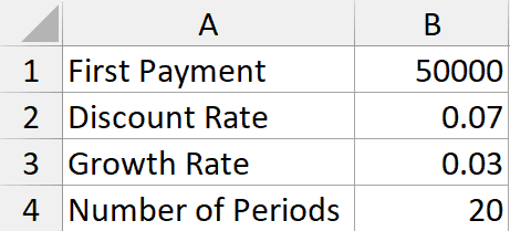
Below is the data that I have put in Excel.

Where:
- B1 is the first payment (C1) = 50000
- B2 is the discount rate (r) = 7%
- B3 is the growth rate (g) = 3%
- B4 is the number of periods (n) = 20
Here is the formula for the present value of the growing annuity:
=B1/(B2-B3)*(1-((1+B3)/(1+B2))^B4)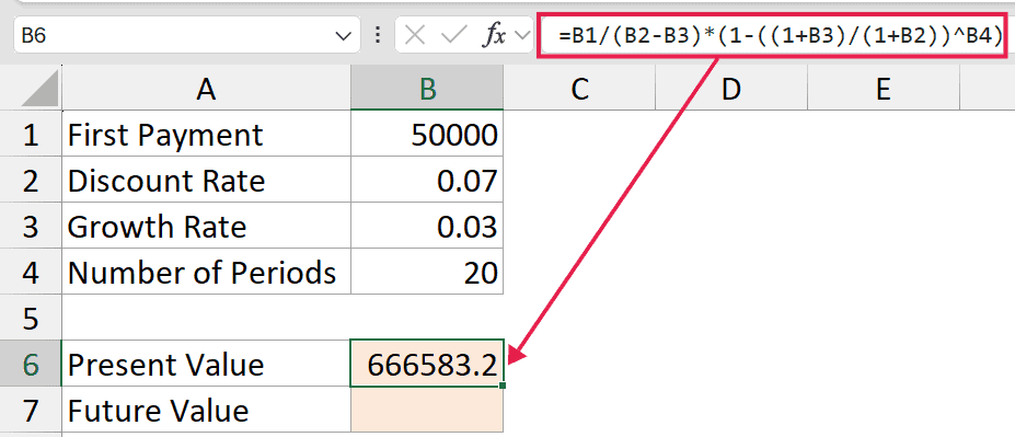
Here is the formula for the future value of the growing annuity:
=B1*((1+B2)^B4-(1+B3)^B4)/(B2-B3)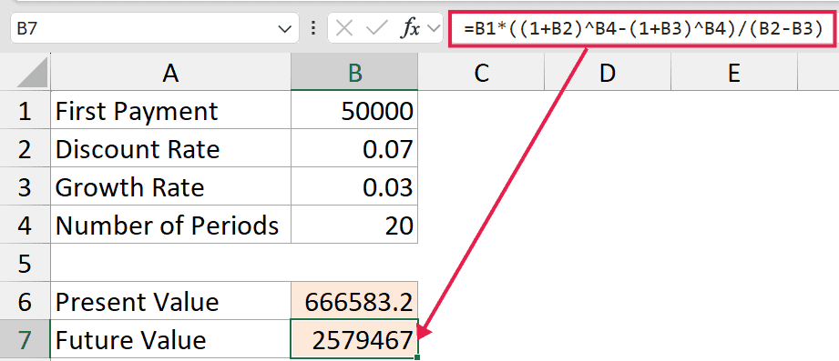
Where:
- B1 is the first payment (C1) = 50000
- B2 is the discount rate (r) = 7%
- B3 is the growth rate (g) = 3%
- B4 is the number of periods (n) = 20
How do these formulas work?
The PV formula takes your first payment and divides it by the difference between the discount rate and growth rate. That gives you the value if the payments went on forever (a growing perpetuity).
Then it multiplies that by (1 − ((1 + g) / (1 + r))^n), which scales it down to only count n periods instead of forever.
The FV formula works a bit differently.
It takes each payment, grows it forward at the discount rate until the end of period n, and adds them all up. The closed-form version just does all that in one step.
For the pension example, you should get a PV of around $666,577 and an FV of around $2,579,467. That means the pension is worth roughly $666,000 today, and if you reinvested every payment at 7%, you’d end up with about $2.58 million after 20 years.
Method 2: Building a Period-by-Period Schedule
The direct formula is great for a quick answer.
But if you want to actually see each payment, or if you need to verify the numbers, a period-by-period schedule is the way to go.
This method is also useful when the growth rate equals the discount rate. The direct formula breaks down in that case, and I’ll explain why later.
Let’s build the schedule for the same pension example.
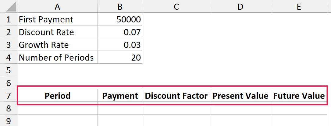
Here are the steps to build the schedule:
- In cell A7, enter the header Period. In B7, enter Payment. In C7, enter Discount Factor. In D7, enter Present Value.
Note: I decided to create this table right below my dataset, but if you want, you can also create this in another worksheet.
- In cell A8, type 1. Drag this down to A27 to get periods 1 through 20.
- In cell B8, enter the formula for the first payment:
=$B$1*(1+$B$3)^(A8-1)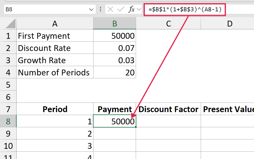
- Copy this formula down to B27. This gives you each year’s payment, growing at 3% every year.
- In cell C8, enter the discount factor formula:
=1/(1+$B$2)^A8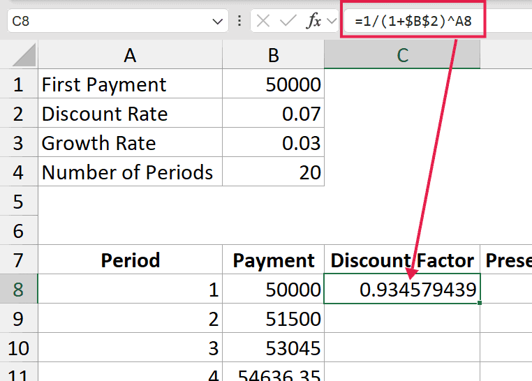
- Copy this down to C27. This is the factor you multiply each payment by to get its present value.
- In cell D8, enter:
=B8*C8- Copy this down to D27.
- In any empty cell (say D28), sum the Present Value column:
=SUM(D8:D27)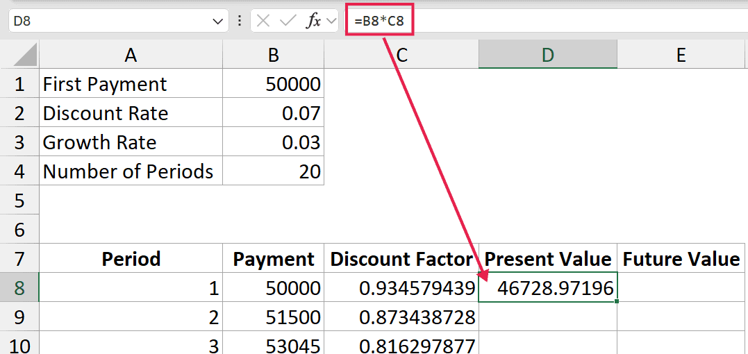
The total in cell D28 should match the PV you got from the direct formula in Method 1.
For FV, you can do the same thing, but instead of discounting each payment back, you compound each one forward to the end of period 20. The formula in a new column would be:
=B8*(1+$B$2)^($B$4-A8)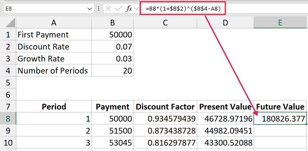
Sum that column, and you have your future value.
The advantage of this method is that you can actually see each year’s payment and how much it contributes to the final value. Useful if you want to double-check the math or share the workings with someone else.
Handling Special Cases
The formulas in Method 1 assume r ≠ g. Here’s what to do when things are a bit different.
When the Growth Rate Equals the Discount Rate
If r = g, the direct formula gives you a divide-by-zero error. In that case, the math simplifies:
Present Value (when r = g):
=B1*B4/(1+B2)Future Value (when r = g):
=B1*B4*(1+B2)^(B4-1)You can also handle this automatically with an IF check:
=IF(B2=B3, B1*B4/(1+B2), B1/(B2-B3)*(1-((1+B3)/(1+B2))^B4))That way, your calculator works no matter what the user enters.
Growing Perpetuity (Payments Go on Forever)
If the payments continue indefinitely (like a dividend on a stock that never stops), you have a growing perpetuity. The formula for that is called the Gordon Growth Model:
=B1/(B2-B3)This only works if the discount rate is greater than the growth rate. If g ≥ r, the value is infinite, which is not a real-world situation.
Annuity Due (Payments at the Start of the Period)
All the formulas above assume the payment comes at the end of each period (ordinary annuity). If the payment comes at the start of each period (annuity due), just multiply the PV or FV result by (1 + r).
=B6*(1+B2)This applies the extra period of discounting (or compounding) that an annuity due gets.
Things to Keep in Mind
- Match your rate period to your payment period. If payments are monthly, use a monthly discount rate and a monthly growth rate. The formulas don’t care about annual vs. monthly, but you have to be consistent. A common mistake is using an annual discount rate with monthly payments, which gives a wildly wrong answer.
- Check that the formula assumes the right payment timing. The standard formula assumes end-of-period payments. If your payments come at the start of each period, multiply the result by
(1 + r)to convert it.
- Watch out for
g ≥ rin the perpetuity case. For a growing perpetuity, the discount rate must be greater than the growth rate. Otherwise, the formula gives a negative or infinite number, which makes no economic sense.
- The first payment is C1, not C0. The formula uses the payment at the end of period 1 as the starting point. If someone gives you the payment today (C0) with growth from that, the first payment in the formula is
C0 × (1 + g), not justC0.
- Double-check with the schedule method. If you’re unsure whether your direct formula is right, build the period-by-period schedule and compare. They should match to the dollar.
In this article, I covered the direct formula, the period-by-period schedule, and how to turn the two into a reusable calculator.
The special cases (when the growth rate equals the discount rate, growing perpetuities, and annuity due) will come up often enough once you start using this, so it’s worth keeping them in mind.
I hope you found this article helpful.
Other Excel articles you may also find helpful:


