

If you want a formula that builds its own cell reference out of text, like a sheet name typed in a cell or an address you piece together, the INDIRECT function is what you need.
It takes a text string and turns it into a real, working reference to a cell or a range.
One thing to know up front. INDIRECT does not spill. It returns a single reference per call, and it is a volatile function, so it recalculates every time anything on the sheet changes.
In this article, I’ll show you how to use INDIRECT with a few practical examples.
INDIRECT Syntax
Here is the syntax of the INDIRECT function:
=INDIRECT(ref_text, [a1])
- ref_text – the text string that describes the reference you want. This can be a cell address like “B2”, a range like “C2:C7”, a sheet reference like “Jan!B2”, or a named range. If the text is not a valid reference, INDIRECT returns a #REF! error.
- a1 – an optional logical value that tells INDIRECT which reference style the text uses. Leave it out or set it to TRUE for the normal A1 style. Set it to FALSE to read the text as an R1C1 style reference.
When to Use the INDIRECT Function in Excel
Use INDIRECT when you need to:
- Turn a text address into a live reference, so the address can come from another cell or be built with a formula.
- Pull data from a sheet whose name sits in a cell, which is handy for summary dashboards.
- Keep a reference fixed in place even when rows or columns are inserted around it.
- Drive dependent drop-down lists off named ranges.
Let me show you how this works with a few practical examples.
Example 1: Reference a Cell From a Text Address
Let’s start with the simplest case.
Below is a small summary table. Column A has the metric name and column B has its value.
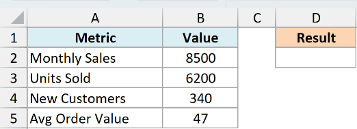
I want to pull the value from cell B2 by describing that cell as plain text.
Here is the formula:
=INDIRECT("B2")
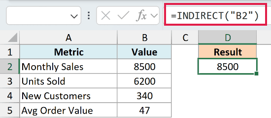
Here, INDIRECT takes the text string “B2”, reads it as an address, and returns what is actually in B2, which is 8500.
On its own this looks pointless, since you could just type =B2. The value comes when that text is not hard-coded but sits in a cell or gets built by a formula, which is what the next examples do.
Example 2: Build a Reference From Parts to Fetch Any Row
Here’s where INDIRECT starts to earn its keep.
Below is a price list. Column A has the product and column B has its price, running from row 2 to row 6.
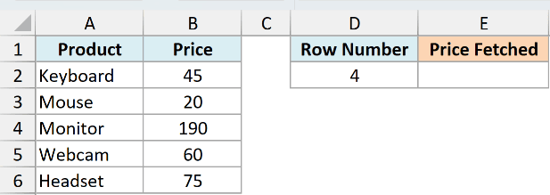
I want to type a row number in cell D2 and have the formula fetch the price from that row automatically.
Here is the formula:
=INDIRECT("B"&D2)
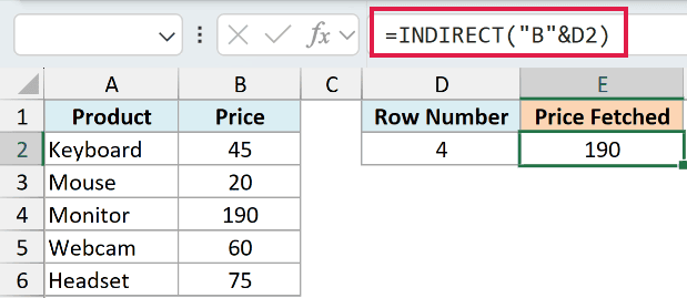
In the above formula, the text “B” is joined to the number in D2 using the ampersand. With 4 in D2, that builds the string “B4”, and INDIRECT turns it into a reference to cell B4, returning 190.
Change D2 to any other row number and the result updates on its own. This is a simple way to fetch a value by position without VLOOKUP or INDEX.
Example 3: Pull Data From a Sheet Named in a Cell
This next one is something I use often for summary dashboards that reference data from another sheet.
Say you have a separate sheet for each month, named Jan, Feb, and Mar, and each of those sheets holds that month’s total revenue in cell B2. On a dashboard sheet, cell A2 holds the month name you want to look at.
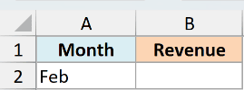
I want the dashboard to pull the revenue from whichever sheet is named in A2, without editing the formula each time.
Here is the formula:
=INDIRECT("'"&A2&"'!B2")
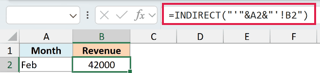
How this formula works:
- “‘”&A2&”‘” wraps the sheet name from A2 in single quotes, so a name with spaces (like “Q1 Data”) still works.
- &”!B2″ adds the cell you want from that sheet.
- With Feb in A2, the string becomes ‘Feb’!B2, and INDIRECT returns 42000, the value sitting in Feb!B2.
Switch A2 to Jan or Mar and the dashboard reads from that sheet instead. One formula covers every month.
Pro Tip: The single quotes around the sheet name are only strictly needed when the name has spaces, but leaving them in always is a safe habit so your formula never breaks the day someone renames a sheet to “Sales Data”.
Example 4: Lock a Range So Inserting Rows Doesn’t Shift It
Here’s a subtle one that saves a lot of broken totals.
Below is a list of monthly expenses in the range B2:B7.
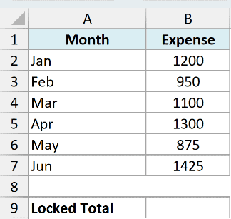
I want a total that always sums B2:B7, even if someone inserts a new row above the range.
Here is the formula:
=SUM(INDIRECT("B2:B7"))
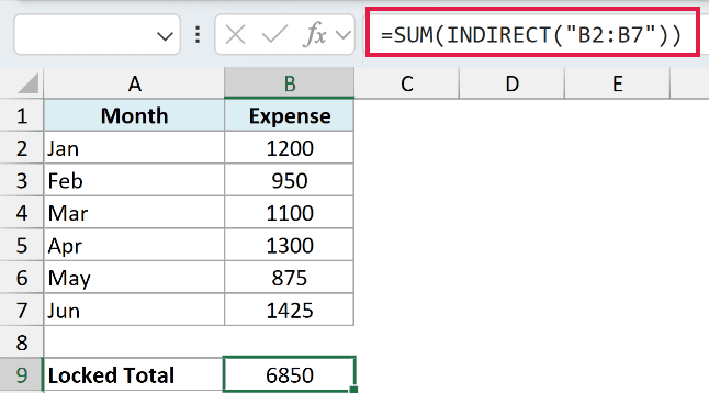
This returns 6850, the total of the six values.
A normal =SUM(B2:B7) adjusts itself when you insert or delete rows around it, shifting to follow the data to a new address like B3:B8.
Because INDIRECT reads “B2:B7” as plain text, Excel never rewrites it. The total stays pinned to those exact cell addresses no matter what you insert around them.
Example 5: Average a Named Range Chosen by Text
Here’s a clean one that shows off how INDIRECT reads named ranges.
Below is a table of marks for five students across three subjects. Column B holds the Math scores, column C the Physics scores, and column D the Chemistry scores.
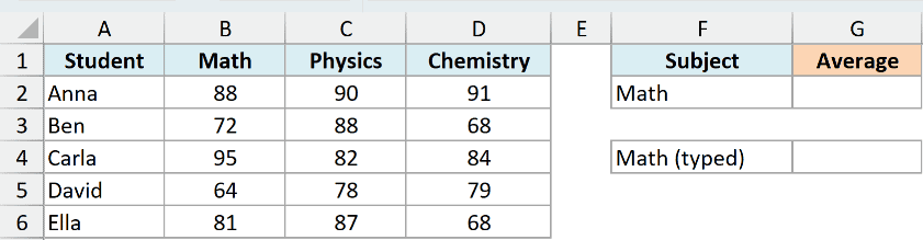
I’ve named B2:B6 as Math, C2:C6 as Physics, and D2:D6 as Chemistry. I want the average Math score by passing that range name in as plain text.
Here is the formula:
=AVERAGE(INDIRECT("Math"))
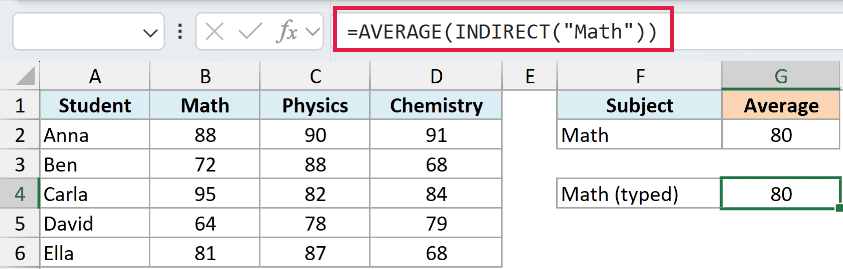
INDIRECT reads the text “Math” as the name of a range, so it hands back the reference B2:B6. AVERAGE then works on those five scores and returns 80.
The real payoff is driving the subject from a cell. Put the subject name in F2 and point INDIRECT at that cell instead.
=AVERAGE(INDIRECT(F2))
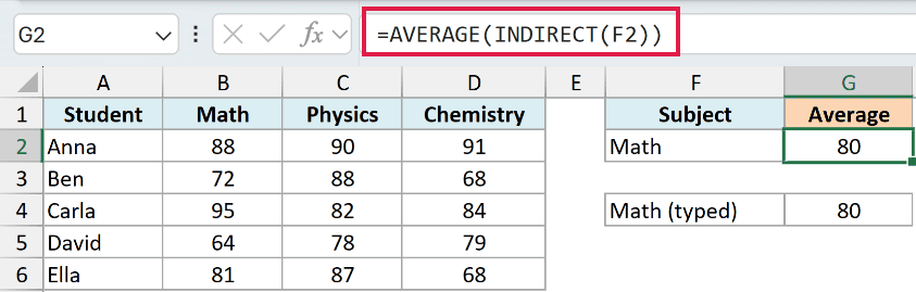
With Math in F2, this returns 80. Type Physics or Chemistry into F2 and the same formula switches to that subject’s range and recalculates, no editing needed.
Pro Tip: The range name here is not in quotes because F2 already holds it as text. Only wrap a name in quotes when you type it straight into the formula, like “Math” in the first version.
Example 6: Create Dependent Drop-Down Lists With INDIRECT
This is probably the most popular use of INDIRECT, and it makes data entry a lot cleaner.
Say you have three category lists set up as columns: Fruits (Apple, Banana, Mango), Vegetables (Carrot, Potato, Onion), and Dairy (Milk, Cheese, Yogurt). You want a category drop-down in E2 and a second drop-down in F2 that only shows items from the chosen category.
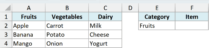
First, create one named range for each category, with the range name matching the header exactly, so a range named Fruits holds Apple, Banana, and Mango. Then set up the first drop-down in E2 with the three category names.
Now build the dependent drop-down in F2:
- Select cell F2.
- Go to the Data tab and click Data Validation.
- Under Allow, choose List.
- In the Source box, enter the formula below, then click OK.
=INDIRECT($E$2)
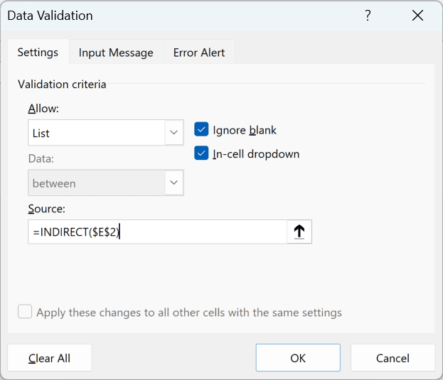
Now when E2 shows Fruits, INDIRECT turns that text into a reference to the named range Fruits, so the F2 drop-down lists only Apple, Banana, and Mango.
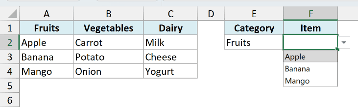
Pick Dairy in E2 instead and the F2 drop-down switches to Milk, Cheese, and Yogurt.
Pro Tip: Named ranges can’t contain spaces, so a category like “Frozen Foods” would break this. Name the range Frozen_Foods and use =INDIRECT(SUBSTITUTE($E$2,” “,”_”)) as the source, which swaps the space for an underscore before INDIRECT reads it.
Example 7: Reference R1C1 Style With the a1 Argument
For the last example, let’s use the optional a1 argument.
Below is a small grid of values in A1:C3. Cell E2 holds a row number and F2 holds a column number.

I want to fetch a value using those row and column numbers directly, which the R1C1 style is built for.
Here is the formula:
=INDIRECT("R"&E2&"C"&F2,FALSE)
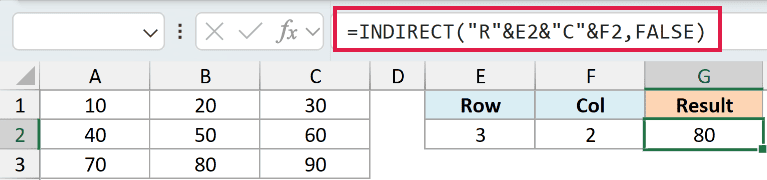
Here, the a1 argument is set to FALSE, which tells INDIRECT to read the text as an R1C1 reference (R for row, C for column).
With 3 in E2 and 2 in F2, the string becomes “R3C2”, meaning row 3, column 2, so INDIRECT returns 80, the value in cell B3.
This is the neat part of R1C1 style. Because the column is a number, you can build it from a cell just like the row, which is awkward to do with normal column letters.
Tips & Common Mistakes
- INDIRECT is volatile. It recalculates every time anything on the sheet changes, not just when its own inputs change. A handful of INDIRECT formulas is fine, but hundreds of them can noticeably slow a large workbook, so use it only where you actually need a text-driven reference.
- Renaming breaks it silently. A normal reference updates itself when you rename a sheet or a named range. INDIRECT does not, because it only sees text. Rename a sheet from Feb to February and any =INDIRECT(“Feb!B2”) turns into a #REF! error.
- It can’t read a closed workbook. INDIRECT can only pull from a workbook that is currently open. Point it at a closed file and it returns #REF!, unlike normal external references that can read a closed source.
- Watch for #REF! errors. If the text doesn’t resolve to a valid reference (a typo in the address, a missing named range, or missing quotes around a sheet name with spaces), INDIRECT returns #REF!. Check the text string first when troubleshooting.
INDIRECT is one of those functions that looks odd until the moment you need it.
Once you do, it is the cleanest way to turn text into a live reference, whether that text is a sheet name on a dashboard, an address you build with a formula, or the source behind a dependent drop-down list.
Try it on your own data with the examples above and it will quickly make sense.
Other Excel Articles You May Also Like:
